
PyT
A Static Analysis Tool for Detecting Security Vulnerabilities in
Python Web Applications
Master’s Thesis
Stefan Micheelsen, Bruno Thalmann
Aalborg University
Computer Science
This report is written using L
A
T
E
X in GNU Emacs. Figures are made using dot, Tikz and
PyT. For screen-shots Snipping Tool and Shutter have been used.

Title:
PyT - A Static Analysis Tool for Detect-
ing Security Vulnerabilities in Python
Web Applications
Theme:
Static Analysis, Web Application Secu-
rity
Project Period:
Spring Semester 2016
Project Group:
des106f16
Participant(s):
Stefan Micheelsen
Bruno Thalmann
Supervisor(s):
René Rydhof Hansen
Mads Chr. Olesen
Page Numbers: 101
Date of Completion:
May 31, 2016
Abstract:
The amount of vulnerabilities in soft-
ware grows everyday. This report ex-
amines vulnerabilities in Flask web
applications, which is a Python web
framework. Cross site scripting, com-
mand injection, SQL injection and path
traversal attacks are used as example
vulnerabilities. A static analysis of
Python is used to analyse the flow of
information in the given program. The
static analysis consists of constructing
a control flow graph using polyvariant
interprocedural analysis. The fixed-
point theorem is used for analysing
the control flow graph. Using an ex-
tended version of the reaching defi-
nitions it is possible to capture infor-
mation flow through a program. A
tool has been implemented and can be
used on whole projects giving possi-
ble vulnerabilities as output. At last an
evaluation of the tool is presented. All
example vulnerabilities were detected
and real world projects were success-
fully used as input.
Source code:
The content of this report is freely available, but publication (with reference) may only be pursued due to
agreement with the author.
Summary
This report presents the static analysis too PyT which has been created to detect
security vulnerabilities in Python web applications, in particular applications built
in the framework Flask.
The tool utilizes the monotone framework for the analysis. An AST is built by
the builtin AST library, and a CFG is built from the AST. The resulting CFG is then
processed so Flask specific features are taken into account. A modified version
of the reaching definitions algorithm is now run by the fixed-point algorithm to
aid the finding of vulnerabilities. Vulnerabilties are detected based on a definition
file containing ’trigger words’. A trigger word is a word that indicate where the
flow of the program can be dangerous. The detected vulnerabilities are in the end
reported to the developer.
PyT has been created with flexibility in mind. The analysis can be either
changed or extended so the performance of PyT can be improved upon. Also
the Flask specific processing can be changed so other frameworks can be analysed
without major changes to PyT.
In order to test the abilities of PyT a number of vulnerable applications was
manufactured and PyT was evaluated with these. All the manufactured examples
was correctly identified as being vulnerable by PyT.
To test PyT in a more realistic setting it was also run on 7 open source projects.
Here no vulnerabilities were found. One of the projects was so big that PyT spent
very long on the analysis and was therefore terminated.
v
Preface
This master’s thesis has been prepared by 10th semester Software Engineering
students at Aalborg University, during the spring-semester of 2016. It is expected
of the reader to have a background in IT/software, due to the technical content.
References and citations are done by the use of numeric notation, e.g. [1], which
refers to the first item in the bibliography.
We would like to thank our supervisor René Rydhof Hansen and co-supervisor
Mads Chr. Olesen for their excellent supervision throughout the project period.
Aalborg University, May 31, 2016
vii
Contents
Preface vii
1 Introduction 1
2 Preliminaries 3
2.1 Existing Tools . . . . . . . . . . . . . . . . . . . . . . . . . . . . . . . . 3
2.1.1 Python Taint Mode . . . . . . . . . . . . . . . . . . . . . . . . . 3
2.1.2 Rough Auditing Tool for Security . . . . . . . . . . . . . . . . 4
2.1.3 Comparison . . . . . . . . . . . . . . . . . . . . . . . . . . . . . 4
2.2 Related Work . . . . . . . . . . . . . . . . . . . . . . . . . . . . . . . . 4
2.2.1 Balancing Cost and Precision of Approximate Type Inference
in Python . . . . . . . . . . . . . . . . . . . . . . . . . . . . . . 4
2.3 Python Web Frameworks . . . . . . . . . . . . . . . . . . . . . . . . . 5
2.3.1 Django . . . . . . . . . . . . . . . . . . . . . . . . . . . . . . . . 5
2.3.2 Flask . . . . . . . . . . . . . . . . . . . . . . . . . . . . . . . . . 6
2.4 Why Flask . . . . . . . . . . . . . . . . . . . . . . . . . . . . . . . . . . 6
3 Python 7
3.1 Python . . . . . . . . . . . . . . . . . . . . . . . . . . . . . . . . . . . . 7
3.1.1 About Python . . . . . . . . . . . . . . . . . . . . . . . . . . . . 7
3.1.2 Parsing Python . . . . . . . . . . . . . . . . . . . . . . . . . . . 7
3.1.3 Objects . . . . . . . . . . . . . . . . . . . . . . . . . . . . . . . . 8
3.1.4 Collections . . . . . . . . . . . . . . . . . . . . . . . . . . . . . . 8
3.1.5 Control Structures . . . . . . . . . . . . . . . . . . . . . . . . . 9
3.1.6 Decorators . . . . . . . . . . . . . . . . . . . . . . . . . . . . . . 12
3.1.7 Import . . . . . . . . . . . . . . . . . . . . . . . . . . . . . . . . 13
3.2 Parameter Passing . . . . . . . . . . . . . . . . . . . . . . . . . . . . . 14
3.3 Surprising Features in Python . . . . . . . . . . . . . . . . . . . . . . . 16
3.3.1 While - Else . . . . . . . . . . . . . . . . . . . . . . . . . . . . . 16
3.3.2 Generator Expression . . . . . . . . . . . . . . . . . . . . . . . 17
ix
x Contents
4 Flask 19
4.1 Flask . . . . . . . . . . . . . . . . . . . . . . . . . . . . . . . . . . . . . 19
5 Security Vulnerabilities 23
5.1 Injection Attacks . . . . . . . . . . . . . . . . . . . . . . . . . . . . . . 23
5.1.1 SQL Injection . . . . . . . . . . . . . . . . . . . . . . . . . . . . 23
5.1.2 Command Injection . . . . . . . . . . . . . . . . . . . . . . . . 25
5.2 XSS . . . . . . . . . . . . . . . . . . . . . . . . . . . . . . . . . . . . . . 25
5.3 Path Traversal . . . . . . . . . . . . . . . . . . . . . . . . . . . . . . . . 26
5.4 Detecting Vulnerabilities . . . . . . . . . . . . . . . . . . . . . . . . . . 27
6 Theory 29
6.1 General Example . . . . . . . . . . . . . . . . . . . . . . . . . . . . . . 30
6.2 Control Flow Graph . . . . . . . . . . . . . . . . . . . . . . . . . . . . 30
6.2.1 Interprocedural Analysis . . . . . . . . . . . . . . . . . . . . . 31
6.3 Lattice . . . . . . . . . . . . . . . . . . . . . . . . . . . . . . . . . . . . 36
6.4 Monotone Functions . . . . . . . . . . . . . . . . . . . . . . . . . . . . 38
6.5 Fixed-point . . . . . . . . . . . . . . . . . . . . . . . . . . . . . . . . . . 38
6.6 Systems of Equations . . . . . . . . . . . . . . . . . . . . . . . . . . . . 39
6.7 Dataflow Constraints . . . . . . . . . . . . . . . . . . . . . . . . . . . . 39
6.8 The Fixed-point Algorithm . . . . . . . . . . . . . . . . . . . . . . . . 40
6.9 Dataflow Analysis . . . . . . . . . . . . . . . . . . . . . . . . . . . . . . 41
6.9.1 Reaching definitions . . . . . . . . . . . . . . . . . . . . . . . . 41
6.10 Taint Analysis . . . . . . . . . . . . . . . . . . . . . . . . . . . . . . . . 44
6.11 Analysis Extension . . . . . . . . . . . . . . . . . . . . . . . . . . . . . 45
6.11.1 Propagation of Reassignments . . . . . . . . . . . . . . . . . . 45
6.11.2 Assignment of Variable Derivations . . . . . . . . . . . . . . . 46
6.12 Finding Vulnerabilities . . . . . . . . . . . . . . . . . . . . . . . . . . . 46
7 Implementation 49
7.1 Handling Imports . . . . . . . . . . . . . . . . . . . . . . . . . . . . . . 51
7.2 Abstract Syntax Tree . . . . . . . . . . . . . . . . . . . . . . . . . . . . 52
7.3 Control Flow Graph . . . . . . . . . . . . . . . . . . . . . . . . . . . . 54
7.3.1 From AST to CFG . . . . . . . . . . . . . . . . . . . . . . . . . 54
7.3.2 Visitor implementation . . . . . . . . . . . . . . . . . . . . . . 55
7.4 Framework adaptor . . . . . . . . . . . . . . . . . . . . . . . . . . . . . 56
7.5 Flexible analysis . . . . . . . . . . . . . . . . . . . . . . . . . . . . . . . 57
7.5.1 Implementing Liveness . . . . . . . . . . . . . . . . . . . . . . 57
7.6 Vulnerabilities . . . . . . . . . . . . . . . . . . . . . . . . . . . . . . . . 58
7.6.1 Taint Analysis . . . . . . . . . . . . . . . . . . . . . . . . . . . . 58
7.6.2 Sources, Sinks and Sanitisers in Flask . . . . . . . . . . . . . . 59
7.6.3 Trigger Word Definition . . . . . . . . . . . . . . . . . . . . . . 61
Contents xi
7.6.4 Finding and Logging Vulnerabilities . . . . . . . . . . . . . . . 61
7.7 PyT . . . . . . . . . . . . . . . . . . . . . . . . . . . . . . . . . . . . . . 62
7.7.1 Positional Arguments . . . . . . . . . . . . . . . . . . . . . . . 62
7.7.2 Optional Arguments . . . . . . . . . . . . . . . . . . . . . . . . 62
7.7.3 Command Line Argument Summary . . . . . . . . . . . . . . 63
7.8 Testing . . . . . . . . . . . . . . . . . . . . . . . . . . . . . . . . . . . . 65
7.9 Limitations . . . . . . . . . . . . . . . . . . . . . . . . . . . . . . . . . . 67
7.9.1 Dynamic Features . . . . . . . . . . . . . . . . . . . . . . . . . 67
7.9.2 Decorators . . . . . . . . . . . . . . . . . . . . . . . . . . . . . . 68
7.9.3 Libraries . . . . . . . . . . . . . . . . . . . . . . . . . . . . . . . 68
7.9.4 Language Constructs . . . . . . . . . . . . . . . . . . . . . . . . 68
8 Discussion 71
8.1 Evaluation . . . . . . . . . . . . . . . . . . . . . . . . . . . . . . . . . . 71
8.1.1 Detecting Manufactured Vulnerabilities . . . . . . . . . . . . . 71
8.1.2 Detecting Vulnerabilities in Real Projects . . . . . . . . . . . . 75
8.2 Reflections . . . . . . . . . . . . . . . . . . . . . . . . . . . . . . . . . . 75
8.2.1 Are Frameworks like Flask Good for Web Security? . . . . . . 75
8.3 Future Works . . . . . . . . . . . . . . . . . . . . . . . . . . . . . . . . 76
8.3.1 Better Trigger Word Definitions . . . . . . . . . . . . . . . . . 76
8.3.2 More Vulnerability Definitions . . . . . . . . . . . . . . . . . . 76
8.3.3 More Efficient Fixed-point Algorithm . . . . . . . . . . . . . . 76
8.3.4 Expanding PyT with Other Analyses . . . . . . . . . . . . . . 77
8.3.5 Support More Frameworks . . . . . . . . . . . . . . . . . . . . 77
9 Conclusion 79
A Vulnerability implementations 81
A.1 SQL injection . . . . . . . . . . . . . . . . . . . . . . . . . . . . . . . . 81
A.2 Command Injection . . . . . . . . . . . . . . . . . . . . . . . . . . . . . 82
A.3 XSS . . . . . . . . . . . . . . . . . . . . . . . . . . . . . . . . . . . . . . 83
A.4 Path Traversal . . . . . . . . . . . . . . . . . . . . . . . . . . . . . . . . 83
B The Abstract Syntax of Python 85
C Flask adaptor implementation 89
D Implementation of the liveness analysis 93
E Trigger word definition for flask 97
Chapter 1
Introduction
Vulnerabilities are being found all the time in software. As new software and
features get published, potential vulnerabilities get released. The attacker has the
advantage in terms of variety of attacks. He can comfortably attempt each attack
in his arsenal while the publisher frantically tries to patch up the breaches. The
publisher often finds out about a vulnerability when it is too late and important
data has been stolen. So the element of surprise is certainly also there. As Bruce
Schneier said:
‘‘Attackers are at an advantage in cyberspace – this will not always be true,
but it’ll certainly be true for the next bunch of years – and that makes defence
difficult.”[1]
Vulnerabilities in web applications There are constantly popping up new tech-
nologies and old ones are evolving and developing new features. These new tech-
nologies and features can be used by the attackers as well. Therefore it is important
to be updated on current and new technologies when developing anything to the
web.[2]
The The OWASP Top Ten Project [3] lists the most critical web application se-
curity flaws. The list is produced by a broad spectrum of security experts. They
recommend that each application is checked for these ten critical security flaws
and each organisation gets aware of how to detect and prevent these flaws.
Considering the difficulty of these problems and the size of code bases in the
average software project, it would be an advantage to have a tool that could help
finding security vulnerabilities. As both of us have an interest in Python develop-
ment we decided to look into tools the could help developing secure Python web
applications. We encountered two Python web frameworks, Django and Flask,
that both do their part in helping the developer. But even though the framework
1
2 Chapter 1. Introduction
helps the developer, it is can still possible to circumvent or overlook these fea-
tures. Therefore we looked into tools that could analyse and find vulnerabilities
in Python code. When examining this type of tools we did not find anything that
satisfied our needs (see Section 2.1) This report will thus create a tool that aids
detection of security flaws in Python web applications, focusing on the Flask web
application framework.

Chapter 2
Preliminaries
In order to analyse a Flask application it is necessary to have a basic understanding
of both the Flask framework and the Python programming language. In addition
we need to have an understanding of the security vulnerabilities that we want to
detect.
This chapter will start out by describing the tools that already exists for finding
security vulnerabilities in Python web applications. Afterwards it will look at
related work performed in this area of research. At last it will examine what web
frameworks exist in order to choose one to focus on throughout the project.
2.1 Existing Tools
In this section we will look at open source tools that find security vulnerabilities by
analysing Python web applications. We have found two tools which are described
in the following.
2.1.1 Python Taint Mode
The Python Taint Mode, Conti and Russo [4], is a library which contains a series
of functions that are used as decorators to taint the source code. To use the library
one has to annotate the source code. Dangerous methods have to be provided with
the and decorators, indicating where untrusted data comes from
and where it can be damaging. Dangerous variables have to be marked with a
function .
Some of these annotations can be provided in the beginning of the file, while
others, like the tainting of variables have to be tainted directly in the code. This
means that one has to go through the whole source code and taint variables and
functions in order to get a proper analysis.
3
4 Chapter 2. Preliminaries
The tool can not handle booleans and has some built in class function it can not
handle. The effectiveness of the tool is not documented.
2.1.2 Rough Auditing Tool for Security
The Rough Auditing Tool for Security(RATS)[5] is a tool for C, C++, Perl, PHP and
Python. It is said to be fast and is good for integrating into a building process. For
Python the tool only checks for risky builtin functions so it is rather basic. Also
RATS has not been developed on since 2013 and the open source project seems
dead.
2.1.3 Comparison
Having found two analysis tools which both are rather different there is not much
to compare. This is because Python Taint Mode requires the developer to decorate
the source code and the RATS tool is checking for builtin functions only. As we
can see there are not many tools and the RATS tool is not even being supported
anymore. This pushed us in the direction of considering to making an open source
tool that finds security vulnerabilities in Python web applications.
2.2 Related Work
As mentioned in Section 2.1, few tools exist that do anything like what we want.
The same is the case in terms of research papers. This section will present the
single paper that had a similar goal as our project.
2.2.1 Balancing Cost and Precision of Approximate Type Inference in
Python
This section contains and overview of the work of Fritz [6]. This master’s thesis
implements a data flow analysis for performing approximate type inference on
Python code.
Fritz [6] builds a CFG of the source code, and uses the worklist algorithm to
compute the result of an analysis using fixpoint iteration. The result is then used
to perform type inference on.
The thesis contains brief explanation about the implementation in Appendix A.
Unfortunately the source code is not available. If the source code would have been
available, the implementation of the control flow graph and the worklist algorithm
could have been used as a foundation for our project.
2.3. Python Web Frameworks 5
2.3 Python Web Frameworks
Before trying to remove security vulnerabilities in applications we needed a frame-
work to focus on. This section contains short descriptions of two of the available
Python web frameworks. The web frameworks were chosen from Web Frameworks
for Python [7]. There are two sets of Python web frameworks, full-stack and non-
full-stack frameworks, one of each was chosen. A full-stack framework is a frame-
work that contains all you need to develop a web application. A non-full-stack
framework is a framework which does not contain all packages to develop a com-
plete web application. Choosing either of these two categories is a matter of taste,
full-stack framework are ready out of the box while non full-stack needs additional
packages, but non-full-stack frameworks have the advantage that the developer
can choose his preferred packages for the job. First the Django web framework
was chosen, which is a full-stack framework. Django was chosen because it is one
of the most popular web frameworks. The second choice was the Flask micro web
framework, one of the most popular non-full-stack frameworks.
2.3.1 Django
Django[8] is a web framework that contains all you need to make a complete
web application. Django is using the Model-View-Controller architecture pat-
tern(MVC)[9]. It is built in a way that forces the developer to add functionality
in a specific way. This means that there is not a lot customisability in the architec-
ture of the project.
Django operates with an abstract concept of apps. An app contains the follow-
ing modules:
• Main module - where the app is starting to execute code.
• Tests module - testing of the app.
• Views module - visualisation of the app.
• Urls module - maps urls to views.
• Models module - models for instance from a database.
• Apps module - nested apps.
A Django web application consists of a combination of apps. The power of Django
is the ease of reuse of an app as they are easily linked together using urls.
6 Chapter 2. Preliminaries
2.3.2 Flask
Flask[10] is a micro web framework. Flask is highly customizable as you can choose
your own architecture of your web application. Also it is possible for instance to
make your own form validation or use a form validation package that one wants.
Flask comes with the following features:
• Development server
• Unit test support
• REST support
The power of Flask is that the developer is able to customise everything.
2.4 Why Flask
This section argues why the the Flask web framework was chosen for this project.
The two key factors was its simplicity and our previous experience with the frame-
work. These factors will be described shortly in the following.
Simplicity The simplicity of Flask enables us to focus on the important task at
hand and not on how to develop a web application. This means rapid development
of web applications used as examples and for testing the tool during the project.
Previous experience The project group has previous experience using Flask. This
again means that we can develop examples faster, without having to spend time
getting acquainted with the framework.

Chapter 3
Python
This chapter contains an overview of the Python programming language, its pa-
rameter passing and some surprising features.
3.1 Python
This section will shortly give an overview of the Python programming language
version 3.5.1. The purpose is to provide a basic knowledge of the programming
language making it possible to follow the Python code used throughout the report.
This section is based on Python 3.5.1 documentation [11].
3.1.1 About Python
The Python programming language is a dynamic, interpreted programming lan-
guage created by Guido van Rossum in the early 1990s. Python supports multiple
programming paradigms, including object oriented and functional programming.
The design philosophy of python values code readability and expressivity.
3.1.2 Parsing Python
A Python program uses newlines as delimiters between statements.
1
But if an
expression is stretched over several lines for instance in parentheses it is still one
line but several physical lines. A comment starts with a “ ” symbol. Indentation is
used for grouping statements for instance a body of a function. A file is a module
which contains definitions and statements and ends with the suffix . A program
can contain several modules.
1
A line can be joined with the next line if it has a “ ” at the end of the line.
7

8 Chapter 3. Python
3.1.3 Objects
All data in Python is represented as objects. An object consists of an identity, a
type and a value. The identity of an object never changes and is represented as
an integer. The type of an object defines how the object can be used and which
operations are supported by the object. The value of an object can for some objects
change. Objects whose value can be changed are called mutable, while objects
whose value can not be changed are immutable.
Definition of objects happen in class definitions. Classes have methods and
attributes attached to it. In Listing 3.1 a class is defined. The method
is an initializer function which is called after a new instance is created of that
class. The keyword references instance variables and instance methods. This
example defines the class which has one instance method and
one instance variable . An instance of this class is created with the value five
passed to the variable through the initializer. The instance method is
then called, which will print the value of .
1
2
3
4
5
6
7
8
9
Listing 3.1: Class definition
3.1.4 Collections
Python contains a number of built in collection classes used to store items in a
structured way. The following will shortly describe the most common collections
and their uses, based on Data structures in Python [12] where additional information
can also be found. The mentioned operations will be exemplified in Listing 3.2.
Lists A list is a mutable sequence of items. A list can be appended and extended
items, and membership testing can be performed with the keyword. A list is
iterable and can be indexed to retrieve individual items. Lists are created with
square brackets or the function.
Tuples A tuple is similar to a list, but is an immutable sequence of a number of
values. A tuple is created with round brackets or the function.

3.1. Python 9
Sets A set is an implementation of the mathematical set. It is an unordered
collection that contains no duplicates. A set is created with curly brackets or the
function.
Dictionaries A dictionary is an associative map, mapping a key to an item. The
key can be any immutable type which can then be extracted as when indexing a
list. Dictionaries are constructed with curly brackets contained key-value pairs or
with the function.
1
2
3
4
5
6
7
8
9
10
11
12
13
14
15
16
17
18
19
20
21
22
23
Listing 3.2: Usage of Python collections
3.1.5 Control Structures
The python programming language has three control structures, , and
. In the following they are presented with simple code examples and a figure
showing the possible information flow through the control structure.
If The control structure has several variants:
1. A simple statement
2. An statement

10 Chapter 3. Python
3. An statement where the statement can be repeated
Figure 3.1 shows a simple control structure containing only one statement.
The code, Figure 3.1a, is an statement with a condition, . If the condition
holds the body is executed and if not, the program moves on to the next piece of
code. This flow is depicted on Figure 3.1b.
1
2
(a) Code example
Entry
if True:
x = 0
Exit
(b) Possible flows
Figure 3.1: A simple control structure containing one statement
The two other variants of the control structure utilise the clause to
define what should be executed if the condition is . This clause can be
a statement body, or a nested which is denoted as an . An example of this
can be seen on Figure 3.2. The outmost has a nested statement which then
contains a body executed when the condition evaluates to and an
executed when it evaluates to .
Note that the else clause is not represented as a independent node, the false
branch is represented in the same way as the true branch in a “if-else” structure.

3.1. Python 11
1
2
3
4
5
6
(a) Code example
Entry
if True:
x = 0 elif False:
Exit
y = 0 z = 0
(b) Possible flows
Figure 3.2: An control structure containing an , an , and an statement
While The control structure has a condition which evaluates to true or
false. If the condition is true the body is executed and the condition is evaluated
again, if it still holds the body is executed again. This process continues until the
condition is false. A control structure can also have an clause. The
body of the clause is executed when the condition of the statement is
false.
An example is displayed in Figure 3.3 which contains a control structure
with the condition and an clause. The possible flows can be seen
on Figure 3.3b, where the clause is executed when the condition resolves to
.
1
2
3
4
5
6
(a) Code example
Entry
while x < 100:
x += 1 x += 3
x += 2 x += 4
Exit
(b) Possible flows
Figure 3.3: A control structure

12 Chapter 3. Python
For The control structure is used for iterating over an object that is iterable.
This could for instance be a list or a tuple. This control structure has an optional
statement, which body is executed when there is nothing to iterate or the
statement is done iterating. To illustrate the control structure we provide two
examples. The first example, on Figure 3.4, shows the most common usage of the
control structure. Here we iterate over a range, which is a built in function that
returns a range of numbers, in this case 0, 1 and 2.
1
2
3
4
(a) Code example
Entry
for x in range(3):
print(x) x = 3
y += 1 Exit
(b) Possible flows
Figure 3.4: A control structure
3.1.6 Decorators
The following is based on Lutz [13, p. 558]. Python contains a syntax that allows
one to transform a function into another function easily. This syntax is called a
decorator and it is denoted with a before a function. A simple decorator
is shown in Listing 3.3. The class implements the method
which is used to save the arguments of the decorator, and the which
is used to replace the original method with a transformation. In this example the
method prints the argument passed to the decorator and then returns the
original function. The output of running this example is presented in Listing 3.4.
Decorators can be used to perform modifications to functions, like preprocessing
some of the arguments or logging the arguments passed to the function.
1
2
3
4
5
6
7
8
9

3.1. Python 13
10
11
12
13
Listing 3.3: Implementation of a simple decorator
1
2
3
Listing 3.4: Output when running the previous example
3.1.7 Import
In Python it is possible to import other modules. Import is possible with the import
statement:
1
Listing 3.5: Import statement.
When using the above import statement the whole module gets imported and
creates a reference to that module in the current namespace. So it imports func-
tions, classes and variables and they can be accessed and used by prefixing with
“module_name”. An example would look like this:
1
2
3
Listing 3.6: Import from statement.
The import statement also has another variant the import-from statement:
1
Listing 3.7: Import from statement.
The import-from statement is importing all names that are defined after the
keyword and adds them to the local namespace. Accessing this module is
different as the names are now in the local namespace one does not need to prefix
them. An example of using a function would look like this:
1
2
3
Listing 3.8: Import from statement.

14 Chapter 3. Python
3.2 Parameter Passing
This section describes how Python deals with parameter passing and is inspired
by Is Python pass-by-reference or pass-by-value? [14], official documentation for this
can be found at Defining Functions [15]. This section is included as it is important
to factor in when parameters are assigned in functions.
The most known parameter passing techniques are pass-by-reference and pass-
by-value. A short description of these two will lead up to an explanation of how
Python is handling parameter passing. Python is basically using pass-by-value but
objects are passed by reference, this is the same as for instance in Java and C#. To
illustrate the different approaches the following two functions are used, Listing 3.9
and Listing 3.10.
1
2
Listing 3.9: Parameter passing: function.
1
2
Listing 3.10: Parameter passing: function.
An abstract way of showing the internal representation will be used. An ex-
ample can be seen on Figure 3.5 where the variable points at a list which is an
object stored in memory as . In python a variable is just a name that points to
some object in memory. A name is illustrated as a box. Assigning ’1’ to a variable
’k’ and then reassigning it to ’2’ does not change the ’1’ in memory. It just creates
the ’2’ object in memory and makes the ’k’ point at this object.
2
l
[0]
Figure 3.5: A variable pointing at a list
Pass-by-reference Pass-by-reference is a parameter passing mechanism where
the argument is directly passed into the function. Consider passing to the
function . After the call the object is changed to: , visualised on
Figure 3.6.
l
[1]
Figure 3.6: The variable pointing at the list after calling function
2
The garbage collector is removing the 1 if it is not used anymore.

3.2. Parameter Passing 15
This is because the variable is passed directly which means that the function
is operating directly on the object. The function behaves similarly, but
because append adds to the list the result is: , visualised in Figure 3.7.
l
[0, 1]
Figure 3.7: The variable pointing at the list after calling function
Pass-by-value The other well known parameter passign mechanism is pass-by-
value, where the actual parameter is copied and passed into the function. The
actual parameter is copied and stored a new place in memory and the copy is
passed into the function. Given the object passed as parameter to the
function , the copied object
0
is changed to:
0
. The original object
remains the same as it is not manipulated by the function.
l
[0]
(a) The variable pointing at the list
after calling the functions
l
0
[1]
(b) The variable
0
pointing at the list
after calling function
Figure 3.8: When reassigning in pass-by-value, only the copied list is changed
A similar thing happens in the function, where after calling the function
and
0
. To visualise see Figure 3.9a and Figure 3.9b, here it
becomes clear that when we access after the call nothing has changed.
l
[0]
(a) The variable pointing at the list
after calling the functions and
l
0
[0, 1]
(b) The variable
0
pointing at the list
after calling function
Figure 3.9: When appending in pass-by-value, only the copied list is changed
Pass-by-object-reference Pass-by-object-reference is the Python way of handling
parameter passing. In this parameter passing mechanism the argument is copied
into a new variable local to the function, but both refer to the same object in mem-
ory. Given the object when calling the function , a new variable
0
is created that refers to the same object in memory. So sets
0
but not because is not manipulating the object but only the name
that is referring to it. Calling manipulates the variables and is visualised
in Figure 3.10a and Figure 3.10b.

16 Chapter 3. Python
l
[0]
(a) The variable pointing at the list
after calling function
l
0
[1]
(b) The variable
0
pointing at the list
after calling function
Figure 3.10: Pass-by-object-reference copies the variable, but points it at the same object as the
original variable
When calling the function the object is referenced and both and
0
are changed to . Calling manipulates the objects referenced by the
variables. This is visualised in Figure 3.11.
l
l
0
[0, 1]
Figure 3.11: The variable and
0
stored in memory as when calling function Listing 3.10.
3.3 Surprising Features in Python
When working so close to the specification of a language some weird or surprising
structures in the language arise. While we programmed the conversion from ab-
stract syntax tree to a control flow graph, we had these experiences once in a while,
and working with the structures has given us some insight, both in the workings of
python and in the details of these interesting structures. This section will discuss
some of these experiences.
3.3.1 While - Else
Normally we know as a simple control structure that has a condition and a
body. The body will execute until the condition is false. This implementation is
also found in Python, but Python has an extra variant of the while loop - an else
clause. An example of a while loop with an else clause can be seen on Figure 3.12a.
The else clause will execute when the condition is false, but if the body is
exited by a statement, the else clause will not be executed. In the example
in Figure 3.12a, this is being utilised to handle values that are unexpected in some
way. If that is the case, we break the body and do not execute the else clause which
contains some logic for the value behaved as expected.

3.3. Surprising Features in Python 17
1
2
3
4
5
6
(a) A while loop with an else clause
Entry
while x < threshold:
if invalid_value(x): handle_value()
x += 1break
Exit
(b) Possible flows
Figure 3.12: An example of a while loop with a break statement
The loop in Python also has an clause which works in the same way.
A example of this can be seen in Figure 3.13.
3.3.2 Generator Expression
The Python language has a goal of being simple, explicit and readable[16]. This can
often be seen in some very elegant constructions contained in the language. One of
those is the generator expression, which was discovered during the development
of PyT.
A generator expression is a concise notation for a common pattern: iterat-
ing over a collection of items and then performing some operation on every el-
ement[17].
1
2
3
4
Listing 3.11: Generator expression, stripping white-space from strings
In Listing 3.11 some file has been parsed into an array. The resulting strings
have some undesirable white-space, and some of the strings are even empty. The
subsequent generator expression handles both of these problems.
A generator expression consists of an expression part and a for part. The for
part is evaluated and the expression is executed on each element of the resulting
iterable. The result is a generator that contains the results.
In Listing 3.11 the generator iterates over the strings with the statement
and filters out empty strings with the statement. The resulting elements are the

18 Chapter 3. Python
1
2
3
4
5
6
(a) Code example
Entry
for x in range(5):
if invalid_value(x): print('Accepted')
print(x)break
Exit
(b) Possible flows
Figure 3.13: A control structure with an statement
stripped of white-space by the initial expression.
The generator in Listing 3.11 can be written without using a generator expres-
sion. This can be seen in Listing 3.12. The generator expression is very clear in
conveying its purpose while being shorter than the “old way”.
1
2
3
Listing 3.12: Listing 3.11 implemented without using an generator expression
Python contains similar constructs called the comprehensions which return a
list, set or dictionary of the element instead of a generator. This construct uses
square or curly parenthesis instead of round parenthesis, but are not different in
any other way. An example of a list comprehension can be seen in Listing 3.13.
1
Listing 3.13: The generator from Listing 3.11 changed to a list comprehension

Chapter 4
Flask
4.1 Flask
Flask is a framework for developing web applications in Python[10]. Its goal is to
be minimal without compromising functionality. It is extensible and flexible, so
components like database and form validation can be chosen by the developer.
The minimal nature of Flask makes it possible to write a web page in a very
small amount of code. The following program, see Listing 4.1, creates a web server
that serves a “Hello World!” page on the root.
1
2
3
4
5
6
7
8
9
Listing 4.1: Minimal Flask application
The Flask framework is imported and a function is defined with the
decorator which tells the framework where to serve the page. The function returns
the string “Hello World!” which is shown on the web page.
The following will present the Flask functionality that will be used in this
project. The descriptions will be based on the Flask Documentation [18].
Routing The decorator is used to bind a function to a URL. The pa-
rameter provided binds the function to the relative path. Example paths are ’/’ for
the root and ’/hello_world’ for a sub-page. The example in Listing 4.1 binds the
function to the url .
19

20 Chapter 4. Flask
HTTP methods Another parameter for the decorator is the meth-
ods allowed. This parameter enables other HTTP methods than the default GET.
An example of enabling the POST method can be seen on Listing 4.2.
1
2
3
4
5
6
Listing 4.2: Enabling POST requests for a login form
Requests Interaction with the incoming request happens through the
object. This object contains all attributes of the request such as arguments from the
query string, form data from POST requests and uploaded files. Listing 4.3 shows
a very simple use of the query string. The query string ’name’ is retrieved with the
default value ’no name’ and assigned to , which is then returned to the user.
1
2
3
4
Listing 4.3: Simple use of the query string
Responses When returning from a function that will be rendered as a web page,
Flask provides several possibilities that makes this process flexible. For example
a returned string will automatically be converted to a valid HTML page. Spe-
cial functions for creating responses exist, such as which
sends a file to the client. HTML files can be rendered with , and
more complex pages can be constructed with the template engine. The template
engine will be explained in the following.
Templates Flask uses a template engine called Jinja2, which helps the devel-
oper keep the application secure. The template engine escapes any dangerous user
inputs without the developer having to consider it.
1
2
3
4
5
Listing 4.4: Rendering a template that displays the name parameter

4.1. Flask 21
1
2
3
4
Listing 4.5: The Jinja2 template used by the hello example
Listing 4.4 shows a simple example of a template being rendered. The
function takes the template displayed in Listing 4.5 and replaces the
name variable with the name entered in the URL. The template engine handles all
escaping, so a malicious user cannot compromise the page through the URL.
The Response object Sometimes a page is more complex than just rendering
a template and replacing variables with the appropriate values. Web pages have
response codes to indicate errors, headers that define the parameters of the request
and cookies to keep track of the user. In order to work with these aspects we need
to get hold of the response before sending it to the client. This is done with the
method. The usage of the method is shown
in Listing 4.6 where a handler for 404 errors is defined. Instead of showing the
browser’s default 404 error, we want to show our own error.
takes a parameter for setting the status code, so creating the custom 404 han-
dler just renders a template and sets the error code to 404. The
method returns a response object, which can then be manipulated by for example
add a header, or a cookie with .
1
2
3
4
5
Listing 4.6: Using make_response to create a custom 404 handler
SQLAlchemy SQL Alchemy is a toolkit for operating on SQL databases directly
from Python. Its goal is to provide “efficient and high performing database access,
adapted into a simple and Pythonic domain language”[19].
The code displayed on Listing 4.7 shows how the connection to a database is
created. The URI of the database is provided to the config attribute of the flask
application, and a database object is created. This object contains a class that
can be used to declare the model. In the example, a model is declared.
1
2
3

22 Chapter 4. Flask
4
5
6
7
8
9
10
11
12
13
14
15
16
Listing 4.7: A SQLAlchemy database model
Now that the database model is created we can populate it. In Listing 4.8 the
usage of a SQLAlchemy database is shown. Between line 1 and line 6 Users are
created and inserted into the database. Afterwards, in line 8, the database is being
queried, first to show all Users, and afterwards to show only the first User named
’admin’.
1
2
3
4
5
6
7
8
9
Listing 4.8: Populating the database and querying the content
Chapter 5
Security Vulnerabilities
To make a tool that finds security vulnerabilities in a program is a very broad and
ambitious task. In order to make the task more manageable we have picked three
common types of vulnerabilities from the OWASP list of top 10 vulnerabilities in
web applications [3]. The chosen vulnerabilities will in the following be described
and code examples will be presented showing the vulnerability in practice. These
code examples will later be used for testing the application.
5.1 Injection Attacks
An injection is an uncontrolled use of user input that reaches an interpreter. This
could be a SQL interpreter, the command line or the Python interpreter. If an
injection vulnerability exists the user can send arbitrary commands to the server,
and possibly access or alter data without authorisation. The typical workaround is
to sanitise the input so only the desired characters will be accepted. [20]
The following will present two subgroups of injection attacks, SQL injections
and command injections.
5.1.1 SQL Injection
This description is based on SQL injection in CWE [21]. SQL injections happen
when an application creates a query partly or entirely from user input without
sanitising this input. The user can escape the query and add an arbitrary query.
Depending on the system, the user can now change the database, read the database
or in severe cases even execute system commands.
Example An implementation of two possible SQL injections can be found in Ap-
pendix A.1. Here a database is setup with the library SQLAlchemy which has
protection against SQL injection built in. The problem is that it also supports raw
23

24 Chapter 5. Security Vulnerabilities
SQL queries, and these examples utilise these. The specific problems of the exam-
ples will be examined in the following.
Naive SQL Handling The first example is a naive handling of SQL queries.
In this example the user has to input the whole query and the query is executed
directly on the database. The method for this is shown on Listing 5.1.
24
25
26
27
28
29
Listing 5.1: An SQL statement is taken as input and executed directly on the database
This is a very unlikely case, but if it gets served by accident, it is a very dangerous
vulnerability.
SQL Filter The second example is where the user has to input the parameter
for the filter method used for filtering the query. The code for the method taking
the parameter as input and querying the database with the filter parameter is
shown on Listing 7.9.
31
32
33
34
35
36
37
38
39
Listing 5.2: A filter string is taken as input and used as a parameter in the filter function.
Because the input string is not sanitised, the user can input whatever he wants,
and an input like
2 or 1 = 1
will return all users in the database, which is of course not intended behaviour.
The key is to insert the keyword which makes another statement possible. The
second statement just has to evaluate to true then all possible database entries are
returned. This ultimately means that the statement sent to the SQL interpreter
looks for all users instead of just a particular one.

5.2. XSS 25
5.1.2 Command Injection
This description is based on Command injection in CWE [22]. Command injec-
tions are very similar to SQL injections, but instead of injecting commands into
a database system, this attack makes it possible to inject commands into server
shell. The ability to perform commands on a server opens up possibilities to read
password files, delete system files and various other dangerous operations.
Example An example of a command injection vulnerable application is presented
in Appendix A.2. In this example a textfile is being used as store for a site where
customers can suggest items for a menu. When customers enter an item into a
textbox, it is stored on a new line in the file. The content of the file is then read
and displayed on the screen, showing all the suggestions. The dangerous function
is shown in Listing 5.3 where it can be seen how the parameter from a textbox is
being passed directly to the shell call in line 18. Entering a string starting with a
command separator (semicolon in bash and ampersand in windows cmd), makes
it possible to interact directly with the system shell. Thus entering a string like
; ls
will print out the contents of folder containing the application. Having access to the
filesystem is obviously dangerous, as a malicious user can now perform arbitrary
commands on the server.
13
14
15
16
17
18
19
20
21
22
23
Listing 5.3: The culprit making command injection possible. Param is not being escaped before
being executed by the shell.
5.2 XSS
Cross site scripting (abbreviated XSS) occur when a site takes untrusted data and
sends it to other users without sanitisation. The description i based on Cross site
scripting in CWE [23]. One example could be a comment section where an evil

26 Chapter 5. Security Vulnerabilities
user sends in a comment containing some JavaScript. When other users see this
comment, their browser runs this JavaScript, which can access cookies or redirect
to a malicious site. Again, this can be prevented by sanitising user input that is
stored.
Example A very simple example of a cross site scripting is presented in Ap-
pendix A.3. The main part is displayed in Listing 5.4. In line 8 some input is taken
and it is inserted into the result page in line 11. A link to the vulnerable web page
can be constructed and sent to a unknowing user who opens the link and gets im-
portant information stolen. In this example the input is not saved permanently, but
if it was saved as for example a comment, a malicious user could inject arbitrary
JavaScript, which all subsequent users would execute in their browsers.
An easy way of avoiding this vulnerability, is to use the template engine of
Flask. If the template engine was used instead of manually replacing the string,
the template engine would sanitise the input.
6
7
8
9
10
11
12
Listing 5.4: The main part of the XSS example from Appendix A.3
5.3 Path Traversal
Path traversal is when access to a resource gives unintended access to the file
system of the server. This description is based on Path traversal in CWE [24]. An
example could be attaching an image to the page decided by some user input. If
the input is not validated an attacker will be able to traverse the file system with
the parent directory element (’..’).
Example An example of this vulnerability can be seen in Appendix A.4. The main
part of the example is displayed in Listing 5.5. Providing the request parameter
as ?image_name=../file.txt will open and show file.txt in the browser. This could
possibly result in database content or passwords to be accessed by intruders.
6
7
8
9

5.4. Detecting Vulnerabilities 27
10
11
Listing 5.5: The main part of the path traversal from Appendix A.4
5.4 Detecting Vulnerabilities
Common for these three security vulnerabilities is that some user input reaches
a sensitive piece of code. An SQL injection happens when user input reaches a
database query Cross site scripting happens when user input reaches some HTML.
Path traversal happens when user input reaches a piece of code that performs file
system access.
To detect these vulnerabilities we need to create a tool that can connect informa-
tion about user input and sensitive code to detect when the operations performed
are dangerous.
Chapter 6
Theory
As we concluded in Section 5.4 we are interested in determining when dangerous
input from a user is able to reach a place in the code where it can cause damage.
A technique for determining this is static analysis where the source of a program
is statically analysed for some property.
This chapter will describe the theory used for building the static analysis engine
used by PyT. It will primarily be based on the lecture notes on static analysis in
Schwartzbach [25].
Undecidable As mentioned above we want to track input and determine whether
it is harmful or not in the way it is used throughout the application. Unfortunately,
it turns out that we will not be able to provide definite answers to this question, but
only qualified approximations. This is due to Rice’s theorem which can be phrased
as “all interesting questions about the behaviour of programs are undecidable” [25,
p. 3]. These interesting questions constitute a rather large group of problems, and
our problem is part of this group.
Static analysis Static analysis is the theoretical topic that engage in solving this
type of problem. The problem is characterised by setting up a number of rules
which define the problem. The program is then converted into a model which
represents the flow of the program. The solution to the problem will then be
gradually approached by an algorithm that applies the defined rules on the model.
The algorithm stops when it can not get closer to an answer. This result is then
the approximation which can be used for further analysis and be the basis of an
answer to the problem.
29

30 Chapter 6. Theory
6.1 General Example
In order to make this theory chapter more understandable an example is intro-
duced which is used throughout this chapter. The code for this example is shown in
Listing 6.1. The example corresponds to the example in Schwartzbach [25] adapted
to Python code.
1
2
3
4
5
6
7
8
9
10
11
Listing 6.1: The general code example used throughout the theory chapter
The program is very simple, it takes some user input which is sent through
a loop that changes the three variables x, y and z, depending on two
statements. The x variable is printed out as the last operation of the program.
Although it is simple it presents some interesting statements and scopes.
6.2 Control Flow Graph
The analysis we want to perform is flow sensitive, meaning that the order of the
statements in the program influence the result of the analysis. When performing a
flow sensitive analysis, a Control Flow Graph (abbreviated CFG for convenience)
can be used to describe the flow of the program.
A CFG is simply just another representation of the program source. It is a
directed graph where a node is a specific place in the program and edges represent
the possible options to which the program can execute to. A CFG always consists
of one entry node and one exit node, called entry and exit. Given a node n the
set of predecessor nodes are denoted pred(n) and the set of successors are denoted
succ(n).
Python control flow graphs CFGs for simple Python statements, such as an as-
signment, have an entry node, a node containing the assignment and an exit node.
The CFG of the sequence of two statements S
1
and S
2
are constructed by deleting
the exit node of S
1
and the entry node of S
2
and gluing the two resulting graphs
together. This process is depicted on Figure 6.1.

6.2. Control Flow Graph 31
Entry
x = 3
Exit
(a) A single statement
Entry
x = 3
y = 5
Exit
(b) A sequence of two statements
Figure 6.1: Construction of a control flow graph for two sequential statements
The CFGs of control flow structures in the Python programming language was
presented in the figures provided in Section 3.1.5.
The CFG for a complete program is produced by systematically combining
the building blocks. A CFG of the general example in Listing 6.1, is shown on
Figure 6.2.
6.2.1 Interprocedural Analysis
As Python contain functions we need a strategy for dealing with these. Schwartzbach
[25] presents two strategies for dealing with this. The first strategy is to analyse a
function when its definition is read in the source code, while the other is to analyse
the function each time it is called.
The first strategy, called monovariant interprocedural analysis, requires that
we assume the worst about every function call, because we cannot know anything
about the context the function is called in.
The second strategy is called polyvariant interprocedural analysis, and pro-
duces a single CFG from a program with a number of function calls. This is done
by gluing the function bodies into the main CFG every time a function is called.
From a source code perspective this would be like in-lining all functions that are
called.
On Figure 6.3 is an example of two CFGs where the first one calls a function,
which is represented by the second CFG. The analysis need to be able to glue these
together without changing the semantics of the program.


6.2. Control Flow Graph 33
Figure 6.3: Two CFGs, one for the calling function and one for the called function. Illustration from
Schwartzbach [25, p. 37]
Shadow variables In order to maintain the correct values for all variables across
scopes we introduce shadow variables. Because parameters of functions have no
relation to the scope of other functions, parameters can be the same for many dif-
ferent function scopes. Shadow variables ensure that the meaning of the different
scopes are kept when gluing the function CFG into the main CFG. The process of
gluing a function into the calling function can be split up into four steps:
• When calling a function all the variables of the current scope need to be
saved, ensuring no clashes with the variables of the function body.
• Then all the formal parameters of the function definition are saved and the
actual parameters are inserted into appropriate variables in order to create
the function local scope.
• The body of the function can now be inserted as it was originally defined,
with the exception that all returns need to be assigned to a unique variable.
• After the function body all the saved variables need to be restored.
The final result is a single CFG for the caller with the callee interwoven in. The
result is depicted on Figure 6.4. Here all the saved variables are characterised with
a prefix and a number i, which is a unique index for the called function.
Adjusting shadow variables to Python The previous description of shadow vari-
ables results in a CFG that simulates the call-by-value parameter passing mecha-
nism. As described in Section 3.2, Python uses call-by-object-reference. We have

34 Chapter 6. Theory
not been able to make an adjustment that captures this completely. Instead we
have made an approximation that ensures that values changed inside a function
will persist after the call.
The modification changes the last of the four steps. Instead of restoring all
saved variables, the variables will be assigned the formal parameter that is being
used inside the function body. In this way the changes made to the formal parame-
ter will persist. This solution is inaccurate because it does not represent reassigning
the parameter correctly (the case in Section 3.2). Instead of being local to
the function body, such a change will persist.
Figure 6.4: The two CFGs glued together with shadow variables. Illustration from Schwartzbach [25,
p. 38]
Polyvariance If we “glue in” the function bodies of called function by referenc-
ing the respective CFG, we get a monovariant analysis. An example of monovariant
analysis can be seen on Figure 6.5a This method puts some limitations on the anal-
yses that are performed on the CFG. For example constant propagation analysis
will be inaccurate because more than one call will be represented in the callee
CFG. For our purposes we need propagation of assignments to be accurate for an
arbitrary number of calls to a function.
The solution is to make the analysis polyvariant. This is done by making mul-
tiple copies of the function body for each call site. This solves the problem about
propagation because every call site has a separate copy of the function where the
analysis can perform unique calculations.


36 Chapter 6. Theory
6.3 Lattice
The static analysis we want to perform utilises the mathematical theory of lattices
together with a monotone function to guarantee that the analysis will terminate.
The theory behind lattices will be described in the following.
Partial orders A lattice is a specialisation of a partial order which will be de-
scribed in the following. A partial order is a mathematical structure L = (S, v)
where S is a set and v is a binary relation where the following conditions are
satisfied:
• Reflexivity: ∀x ∈ S : x v x
• Transitivity: ∀x, y, z ∈ S : x v y ∧ y v z ⇒ x v z
• Antisymmetry: ∀x, y ∈ S : x v y ∧ y v x ⇒ x = y
Least upper bound As the name states, a least upper bound is the least of all
upper bounds. An upper bound y of a set X where X ⊆ S and S is a partial order
is written as X v y. y is an upper bound of X if we have that ∀x ∈ X : x v y.
We can now define the least upper bound, written as tX:
X v tX ∧ ∀y ∈ S : X v y ⇒ tX v y
The greatest lower bound uX can be defined by the same logic.
Lattice A lattice can now be defined as a partial order in which tX and uX is
defined for all X ⊂ S. It should be noted that a lattice must have a unique largest
element > defined as > = tS and unique smallest element ⊥
In Figure 6.6 a lattice with four elements is depicted. These four elements are
deduced from a subset of the general example program on Listing 6.1 (in order to
keep the size of the lattice manageable). The subset can be seen on Listing 6.2.
1
2
3
4
5
6
7
Listing 6.2: The general code example used throughout the theory chapter
This lattice is defined by the set of four expressions {x > 1, x/2, y > 3, x − y}.
In general the set A defines a lattice (2
A
, v) where > = A, ⊥ = ∅, x t y = x ∪ y
and x u y = x ∩ y.

6.3. Lattice 37
{x > 1, x / 2, y > 3, x - y}
{x > 1, x / 2, y > 3} {x > 1, x / 2, x - y} {x > 1, y > 3, x - y} {x / 2, y > 3, x - y}
{x > 1}
{}
{x / 2} {y > 3} {x - y}
{x > 1, x / 2} {x > 1, y > 3} {x > 1, x - y} {x / 2, y > 3} {x / 2, x - y} {y > 3, x - y}
Figure 6.6: A lattice with four expressions.

38 Chapter 6. Theory
Every analysis requires the lattice to contain certain elements of the program in
order to work. Examples range from expressions or assignments to variables. The
presented type of lattice is used in analyses that depend on information about the
expressions in a program. One example of such analysis is ’available expressions’
which is presented in Schwartzbach [25, p. 22]. This analysis finds expressions
that are available at a program point. An available expression is an expression that
has already been calculated earlier in the execution. Finding available expressions
can be used to optimize the program by saving the calculation and thus avoid
recalculating it.
6.4 Monotone Functions
A function f : L → L is monotone when ∀x, y ∈ S : x v y ⇒ f (x) v f (y). Being
monotone does not imply that the function is increasing. All constant functions
are monotone.
If we look at the least upper bound and greatest lower bound as functions they
are monotone in both arguments. This means that we can apply the least upper
bound function on two arguments and be certain that it will never decrease. This
is an important requirement for the fixed-point theorem which will be presented
in the next section.
6.5 Fixed-point
For the static analysis of a program we need a theorem that can find the best ap-
proximation of some dataflow problem. Because we will generally consider prob-
lems that are undecidable, see Chapter 6, we need a framework that overestimate
the answer, and thus makes an approximation.
This framework will be based on the fixed-points theorem which states the
following (quoted from Schwartzbach [25, p. 13]):
Definition 6.1 (Fixed-point theorem)
In a lattice L with finite height, every monotone function f has a unique least
fixed-point defined as
f ix( f ) =
G
i≥0
f
i
( ⊥)
for which f ( f ix( f )) = f ix( f )
The proof of this theorem can be found in Schwartzbach [25, p. 13].
This theorem enables us to find an approximation to an undecidable problem
by walking up the lattice until a fixed-point is reached. This computation has been

6.6. Systems of Equations 39
Figure 6.7: A walk through the lattice, starting a ⊥ and ending in the fixed-point. Illustration from
Schwartzbach [25, p. 13]
illustrated in Figure 6.7 where the analysis starts at ⊥ and end in the fixed-point
which is the approximation to the problem at hand.
6.6 Systems of Equations
Combining equations into a system of equations can be solved by using fixed-
points. Consider an equation system of the form:
x
1
= F
1
(x
1
, . . . , x
n
)
x
2
= F
2
(x
1
, . . . , x
n
)
.
.
.
x
n
= F
n
(x
1
, . . . , x
n
)
Here x
i
are variables and F
i
: L
n
→ L is a monotone function. A least unique
solution to such a system can be found as the least fixed-point of the combined
function F : L
n
→ L
n
defined by:
F(x
1
, . . . , x
n
) = (F
1
(x
1
, . . . , x
n
), . . . , F
n
(x
1
, . . . , x
n
))
6.7 Dataflow Constraints
For analysing a CFG of a program we need to be able to describe the relationship
between the individual nodes. Some analyses track variable content while others
track use of certain expressions. Similarly, some analyses need information from
its successors while others need information from its predecessors.
To describe these different analyses we annotate each node with a dataflow con-
straint. Dataflow constraints relate the value of a node to its neighbouring nodes
and is denoted JvK. A dataflow analysis consists of a number of dataflow con-
straints that each defines the relation of a construction in the programming lan-

40 Chapter 6. Theory
guage.
An example of a dataflow constraint could be conditions (from the liveness
example in Schwartzbach [25])
JvK = JOIN(v) ∪ vars(E)
where JOIN combines the constraints of the successors of v and vars(E) denote
the set of variables occurring in E.
6.8 The Fixed-point Algorithm
A CFG has been defined in Section 6.2 and a lattice has been defined in Section 6.3.
Given a CFG, a lattice and associated dataflow constraints, the fixed-point algo-
rithm can compute the fixed-point. The following is from Schwartzbach [25].
Operating on a CFG that contains the nodes {v
1
, v
2
, . . . , v
n
} we work with the
lattice L
n
. Assuming that the node v
i
generates the dataflow equation Jv
i
K =
F
i
(J v
1
K, . . . , Jv
n
K) , the equations of all the nodes can be combined in a function
F : L
n
→ L
n
.
F(x
1
, . . . , x
n
) = (F
1
(x
1
, . . . , x
n
), . . . , F
n
(x
1
, . . . , x
n
))
This combined function resembles the function presented in Section 6.6, and it
can indeed be solved by fixed-points. A naive algorithm for solving such a function
is presented in Schwartzbach [25]:
1 x = (⊥, . . . , ⊥)
2 do
3 t = x
4 x = F(x)
5 while x 6= t
Algorithm 1: The naive Fixed-Point algorithm as presented in Schwartzbach
[25, p.18 ]
As L
n
is finite and assuming that the constraints that make up F(x) are monotonous,
the fixed-point algorithm will always terminate according to the Fixed-point theo-
rem, see definition 6.1.
There exist more efficient algorithms than the naive version presented, some of
them are described in Schwartzbach [25, p. 18]. Because efficiency was not a high
priority these have not been examined.
6.9. Dataflow Analysis 41
6.9 Dataflow Analysis
The type of dataflow analysis that we want to perform is called the monotone frame-
work. The monotone framework utilises the concepts that have now been intro-
duced.
A CFG of the program is generated to represent the flow of the program. A
lattice with finite height together with a collection of dataflow constraints comprise
the analysis to be performed. Running the fixed-point algorithm on the parts
will result in an approximation of the answer to the analysis which can then be
interpreted.
This section contains a description of the used dataflow analyses.
6.9.1 Reaching definitions
To solve our problem of detecting when unsanitised user input reaches a critical
point in the code, we need an analysis of what assignments may influence the
values of all variables at any point in the program. The Reaching Definitions as
presented in Schwartzbach [25, p. 26] achieves just this.
Consider the Python code from the general example on Listing 6.1. When
executing the program and providing some arbitrary input at line 1, the value will
slide through the control flow of the program until it is printed in the end. At this
point x has been changed by assignments a number of times, and it is not obvious
where the value comes from. By performing the reaching definitions analysis we
can find possible origins of the value.
Performing the analysis As stated earlier a dataflow analysis consist of many
of the concepts that have been introduced until now. These concepts will in the
following be instantiated on the previously introduced example as to present the
complete analysis.
Control flow graph The CFG of this code was presented in Listing 6.1.
The flow of the program is linear until the while loop. The while loop diverts
the flow into the loop and ultimately to the print statement. The loop has two if
statements where the flow is again split up. It is easy to see from the flow graph
that there are many possible routes from entry to exit, and the propagation of
values is not straightforward.
Lattice The lattice used for this analysis is a power set lattice of all the assign-
ments in the program.
L = (2
{x=input(), x=int(x), y=x/2, x=x−y, z=x−4, x=x/2, z=z−1}
, ⊆)
42 Chapter 6. Theory
The lattice of a simplified version of this lattice was described and depicted in
Figure 6.6. Providing an illustration of the full latice would be intangible, but the
structure is similar.
Dataflow Constraint System The analysis is performed backwards by join-
ing the constraints of all predecessors of all nodes. This can be expressed as the
following function:
JOIN(v) =
[
w∈pred(v)
JwK
All nodes other that assignment just join all constraints of their predecessors:
JvK = JOIN(v)
Assignment nodes changes the content of a variable. The former assignment to
this variable will therefore be discarded and replaced with the current assignment
node:
JvK = JOIN(v) ↓ id ∪ {v}
Here the ↓ function removes all assignments to the variable id from the result
of the JOIN.
Applying the previously defined dataflow constraints to the generated CFG
looks as follows:
JentryK = {}
Jx = input()K = JentryK ↓ x ∪ x = input()
Jx = int(x)K = Jx = inputK ↓ x ∪ x = int(x)
Jwhile x > 1K = Jx = int(x)K ∪ Jz = z − 1K
Jy = x/2K = Jwhile x > 1K ↓ y ∪ y = x/2
Jif y > 3K = Jy = x/2K
Jx = x − yK = Jif y > 3K ↓ x ∪ x = x − y
Jz = x − 4K = (Jx = x − yK ∪ Jif y > 3K) ↓ z ∪ z = x − 4
Jif z > 0K = Jz = x − 4K
Jx = x/2K = Jif z > 0K ↓ x ∪ x = x/2
Jz = z − 1K = (Jif z > 0K ∪ Jx = x/2K ↓ z ∪ z = z − 1
Jprint(x)K = Jwhile x > 1K
JexitK = Jprint(x)K
Figure 6.8: Dataflow constraints applied on the generated CFG
6.9. Dataflow Analysis 43
Solving the equation system Solving this system of equations with the fixed-
point algorithm will provide the information we need in order work with our
problem.
The first iteration of this looks as follows:
JentryK = {}
Jx = input()K = {x = input()}
Jx = int(x)K = {x = int(x)}
Jwhile x > 1K = {}
Jy = x/2K = {y = x/2}
Jif y > 3K = {}
Jx = x − yK = {x = x − y}
Jz = x − 4K = {z = x − 4}
Jif z > 0K = {}
Jx = x/2K = {x = x/2}
Jz = z − 1K = {z = z − 1}
Jprint(x)K = {}
JexitK = {}
Figure 6.9: First iteration of the fixed-point algorithm
Here it is clear that only the constraints of assignments have walked up the
lattice, each to the node indicating the flownode itself. After nine iterations all the
assignments will propagate through the program, and the result can be seen on
Figure 6.10. These constraints can now be interpreted in order to answer question
that require knowledge of which assignments reach which nodes.
44 Chapter 6. Theory
JentryK = {}
Jx = input()K = {x = input()}
Jx = int(x)K = {x = int(x)}
Jwhile x > 1K = {x = int(x), y = x/2, x = x − y, x = x/2, z = z − 1}
Jy = x/2K = {x = int(x), y = x/2, x = x − y, x = x/2, z = z − 1}
Jif y > 3K = {x = int(x) , y = x/2, x = x − y, x = x/2, z = z − 1}
Jx = x − yK = {y = x/2, x = x − y, z = z − 1}
Jz = x − 4K = {x = int(x), y = x/2, x = x − y, z = x − 4, x = x/2}
Jif z > 0K = {x = int(x), y = x/2, x = x − y, z = x − 4, x = x/2}
Jx = x/2K = {y = x/2, z = x − 4, x = x/2}
Jz = z − 1K = {x = int(x), y = x/2, x = x − y, x = x/2, z = z − 1}
Jprint(x)K = {x = int(x), y = x/2, x = x − y, x = x/2, z = z − 1}
JexitK = {x = int(x), y = x/2, x = x − y, x = x/2, z = z − 1}
Figure 6.10: Final result of the fixed-point algorithm
Interpreting the result Looking at the final equations the potential flow of values
through the program can be seen. For example, looking at the print statement, the
value of x could have originated from three places in the program: the x = int(x),
x = x − y or the x = x/2 statement. Depending on the purpose of the analysis, this
information can be used to deduce whether any dangerous flows are possible.
6.10 Taint Analysis
The following is based on Schwartz, Avgerinos, and Brumley [26, Part 3]. An
expression which introduces user input in some way is called a source, while a
dangerous destination for such input is called a sink. A function that can neutralise
input so it is not dangerous to send to a sink is called a sanitiser.
Taint analysis is used for tracking the information between sources and sinks.
If some data comes from an untrusted or tainted source it is regarded as being
tainted. All other data is untainted. Which sources introduce taint are defined by
the user of the analysis.
If a taint analysis is marking too much data as tainted, the analysis is overtaint-
ing, while an analysis that is marking too little data as tainted it is undertainting.
If the analysis is neither over- or undertainting it is precise. Undertainting leads to
missing some vulnerabilities while overtainting leads to false positives.
Because finding all vulnerabilities is critical it is common to strive to overtaint-
ing rather than undertainting. This can lead to a problem called taintspread which
is when more and more data is tainted and that with less precision. To help with
that, one can include sanitisers in the analysis which untaints the data.

6.11. Analysis Extension 45
6.11 Analysis Extension
The previously described algorithm is able to detect that a value flows from a
source to a sink. Unfortunately this method is insufficient in finding all vulner-
abilities. When a value from a source is assigned to a variable s, this variable is
not necessarily the one being used when arriving at a sink. Other variables can be
assigned to values that derive from s, or s can be reassigned to a modified version
of s.
These two problems arise from using the method presented in Section 6.9.1.
Two small examples of the problems can be seen in Figure 6.11a and Figure 6.11b.
Here the method is an arbitrary method that introduces taint while is
an arbitrary sensitive sink.
1
2
3
4
5
(a) Reassigning a tainted variable with a
modification of the tainted value
(b) Assigning a derived value of the
tainted variable
In neither of the two examples it will be possible to detect the vulnerability
with the method from Section 6.9.1, because the flow is cut off by the assignments.
To fix this we have introduced two extensions to the method.
6.11.1 Propagation of Reassignments
In order to maintain the tainted variable s ’alive’ we have modified the assignment
dataflow constraint presented in Section 6.9.1. We want to let both the original
assignment as well as the reassignment live in the analysis. First we check if the
current assignment is a reassignment. An assignment is a reassignment if the
variable assigned to also is part of the right hand side. If it is a reassignment, we
omit the arrow function of the original rule, else the rule is as defined originally.
The extended constraint rule is shown below:
JvK = if v is a reassignment:
JOIN(v) ∪ {v}
else:
JOIN(v) ↓ id ∪ {v}

46 Chapter 6. Theory
Now both the original assignment and the reassignment will propagate to the
sink. This modification will still guarantee that the analysis will terminate, because
the analysis will still only walk up the lattice. This is true because the added case
only adds a node to the constraint, which causes the analysis to walk up in the
lattice.
6.11.2 Assignment of Variable Derivations
To be able to detect derivations of variables as being vulnerabilities, we need to
keep track of assignments to these derivations. This will be done when finding
sources in the CFG. Each time a source is found, the subsequent nodes will be
checked for assignments of derivations of this source node. Nodes that fit this
description will be saved together with the source node as a ’secondary’ source
node. When checking for pairs of sources and sinks these assignments will also be
considered as sources.
6.12 Finding Vulnerabilities
Armed with the information provided by the reaching definitions analysis we
should be able to find vulnerabilities in applications. The vulnerabilities men-
tioned in Chapter 5 all have in common that one expression introduces user input
into the program, and a later expression executes this input. The structure of such
application is outlined on Figure 6.12a.
Using the reaching definitions analysis it is possible to determine if the data
obtained at the source will reach the sink, by examining the constraints provided
by the analysis. The secondary nodes mentioned in Section 6.11.2 will likewise
be considered as a source. If the source is contained in the set of constraints of
the sink and the source variable is being used as a parameter by the sink, we can
regard it as a potential security vulnerability.
Such a vulnerability can potentially be harmless because of processing on the
path towards the sink, by a sanitiser. Figure 6.12b shows the outline of an applica-
tion where a sanitiser is used. The flow of such a program makes it impossible to
guarantee that the application is safe, but reporting it to the developer may ease
the process of securing the application.
A sanitised version of the cross site scripting example from Section 5.2 can
be seen in Listing 6.3. The function takes a string input and
returns an escaped version, making it safe to insert into html. PyTwill report this
as a vulnerability, but will add that it may be sanitised by the
function.

6.12. Finding Vulnerabilities 47
entry
. . .
exit
source
. . .
sink
. . .
(a) A vulnerable application
entry
. . .
exit
source
. . .
if x == 1
. . .
sink
. . .
sanitiser
(b) A sanitiser eliminating the vulnerability
Figure 6.12: Control Flow Graphs for applications with potential vulnerabilities
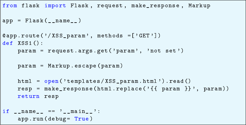
48 Chapter 6. Theory
1
2
3
4
5
6
7
8
9
10
11
12
13
14
15
16
Listing 6.3: The cross site scripting example sanitised by the escape function

Chapter 7
Implementation
This section will give an overview of the different components and the overall flow
of PyT. An illustration giving an abstract overview can be seen on Figure 7.1.
The illustration shows how PyT takes the source code as input, manipulates it
and finally outputs a list of potential vulnerabilities. The process will be described
in the following on a general level.
• The source code is parsed to an abstract syntax tree (denoted as AST) rep-
resentation of each file in the project being analysed. The AST is generated
using the standard Python library [27].
• The AST is systematically traversed and turned into a control flow graph by
the CFG component.
• The resulting CFG is not prepared for the analysis by a framework adaptor,
depending on the web framework used in the source code. The default adap-
tor is the Flask adaptor, but a similar module for Django applications could
be devised.
• The fixed point algorithm is applied on the CFG and the resulting constraints
are annotated on each CFG node The fixed point module is flexible which
means that the analysis can be substituted or extended with other analyses.
By default PyT uses the extended reaching definitions analysis presented in
the previous chapter.
• At last the annotated CFG is investigated, and a log is provided to the user
giving precise information about the potential vulnerabilities found by the
analysis
49

50 Chapter 7. Implementation
Source code
AST
CFG
Framework
Adaptor
Fixed Point
Algorithm
Vulnerabilities
Other
Analysis
Reaching
Definitions
Liveness
Other
Figure 7.1: An abstract overview of the implementation of PyT, showing the main components and
the flow

7.1. Handling Imports 51
7.1 Handling Imports
This section contains a description of how imports are handled when processing
a file. Handling imports is essentially just coupling called functions, class instan-
tiations and variables to the correct definition in another file. As such it is not
theoretically interesting. However, it is a requirement for being able to run PyT
on real projects, which is important because we want to evaluate the security of
complete web applications.
The import statements The two ways of importing in Python, import and import-
from, are presented in Section 3.1.7 and these two ways need to be handled sepa-
rately. When referencing a function in a module imported with the state-
ment the function needs to be prefixed with the name of the module while this is
not the case for .
The file that is given as input to PyT is used as the entry point. First, the
module is used to get what we call local modules and project
modules. A local module is a Python file that is in the same folder as the file. A
project module is a Python file that is in the same project as the file. The project
modules are used to resolve the location of modules placed in another directory.
To illustrate the above consider the following example project structure below.
Consider the entry point being the app.py file. The mod-
ule will construct a list of project modules containing the following modules:
[car_app.app.py, car_app.models.py, car_app.user.forms.py, car_app.user.views.py]. And
a list of local modules containing the modules that are in the same folder as the
entry file: [app.py, models.py].
The module definitions stack Using the module, described in Section 7.2, the
abstract syntax tree(AST) is generated for the entry point. When visiting an import
or import-from node the module and its definitions are loaded. A definition in this
context is a definition of a variable, function or class. A file being loaded usually
also contains imports. In order to control the different import contexts, a module
definition stack is built. Each entry in the stack contains a list of loaded definitions

52 Chapter 7. Implementation
for one file.
To illustrate consider these two modules:
1
2
3
4
5
6
7
8
Listing 7.1: A module that defines a function and two classes called
1
2
3
4
5
6
7
Listing 7.2: A module called importing the above module
First the AST for the entry file is created in this case we say its module . Then
an entry in the stack created for . So the stack contains one module definitions:
stack = [module_definitions<b>].
The AST is visited and when an import statement is visited a new module is
visited and a new module definitions is created and added to the stack. Visiting
the import of results in the following stack: stack = [module_definitions<b>,
module_definitions<a>]
The definitions in the list are: , and . These are added to
the list of module : module_definitions<a> = [ , , ]. Additionally
they are added to the list of module with names prepended with an : mod-
ule_definitions<b> = [ , , ].
This is important so that when one of the imported definitions later is used in
the list of contains the correct definition.
Every time there is an import a new list is added to the stack. When the import
is done the stack is popped. This process handles the names for different modules
and nested imports.
7.2 Abstract Syntax Tree
The module from the standard library in Python is used for building an ab-
stract syntax tree from the source code. This module contains a method that

7.2. Abstract Syntax Tree 53
x = 1
(a) A small Python program
module
[list]
body
assign
0
num
value
[list]
targets
1
n
name
0
'x'
id
store
ctx
(b) The syntax tree of the code in Figure 7.2a
Figure 7.2: A piece of code and the corresponding syntax tree
constructs an AST from a string containing Python code. The abstract grammar
of Python can be found in Appendix B. Selected rules, which are relevant for the
following example, are displayed in Listing 7.3.
1 mod = Module ( stmt ∗ body )
2
3 stmt = Assign ( expr ∗ ta r g e t s , expr value )
4
5 expr = Num( o b j e c t n )
6 | Name( i d e n t i f i e r id , e x p r_context c t x )
Listing 7.3: Selected rules from the Python abstract grammar
Figure 7.2 shows the abstract syntax tree for the small piece of code presented
in Figure 7.2a. The root of the program is the statement which contains a
list of s. In this case this is an which then contains a list of targets
and a value. In this concrete example there is a single target which is the x,
and the value is a with the number 1.

54 Chapter 7. Implementation
7.3 Control Flow Graph
The module contains a class, , that takes an AST and builds a CFG from
it. The CFG is built by traversing the generated AST using the visitor pattern.[28]
The visitor pattern is implemented by the AST module, and our CFG module
utilizes this implementation. The class constructs a list of nodes which
are saved as a .
1
2
3
4
5
6
(a) Code example
I f
t e s t
NameConstant
body
[ Assign ]
o r e l s e
I f
t e s t
NameConstant
body
[ Assign ]
o r e l s e
[ Assign ]
(b) Abstract Syntax Tree
Entry
if True:
x = 0 elif False:
Exit
y = 0 z = 0
(c) Possible flows
Figure 7.3: An AST and the expected CFG
7.3.1 From AST to CFG
Implementing the CFG requires considering all the cases mentioned in Section 3.1.5.
Figure 7.3 shows an one of the cases with the intermediate AST step included (Fig-
ure 7.3b). Here the AST is visualised as a tree, where the first node is an node
1
This node contains a test node, a body, represented as a list of nodes, and an
orelse body, also represented as a list of nodes. In this example the conditions are
nodes and all statements are nodes. The orelse body of the
outer node contains another node which contains the which has the else
in its orelse body.
The CFG of the program is generated by traversing the AST and creating a CFG
node at each node. These nodes are then connected so the resulting CFG reflects
the flow of the program. The implementation of the visitor will be described in
the following.
1
An AST for a complete program starts with a node, but this is not shown here in order
to simplify the tree

7.3. Control Flow Graph 55
7.3.2 Visitor implementation
Listing 7.4 shows the implementation of visiting an AST node. First, another
visitor, the is used to find labels of statements in the CFG. In line 2
it is used to generate the label of the condition in the . Afterwards a CFG node
is created for the condition and appended to the list of CFG nodes. In line 8 the
body of the is handled by the method. This method visits
all nodes in the body and connects them properly. Line 11 now handles and
cases. Again handles the connection of the bodies.
Through the implementation a number of ’last nodes’ are being kept track of.
This is for instance seen in line 13 where the ’last nodes’ of the orelse node are
added to the ’last nodes’ of the body. A ’last statement’ is in this context any
statement that needs to be connected to the subsequent statement of the . Among
these are statements, statements and the last statements of the body,
bodies and the body. These are sent to the calling function by returning
a in line 19. This calling function is which,
as stated above, connects all the nodes properly.
1
2
3
4
5
6
7
8
9
10
11
12
13
14
15
16
17
18
19
Listing 7.4: Visiting an If AST node.
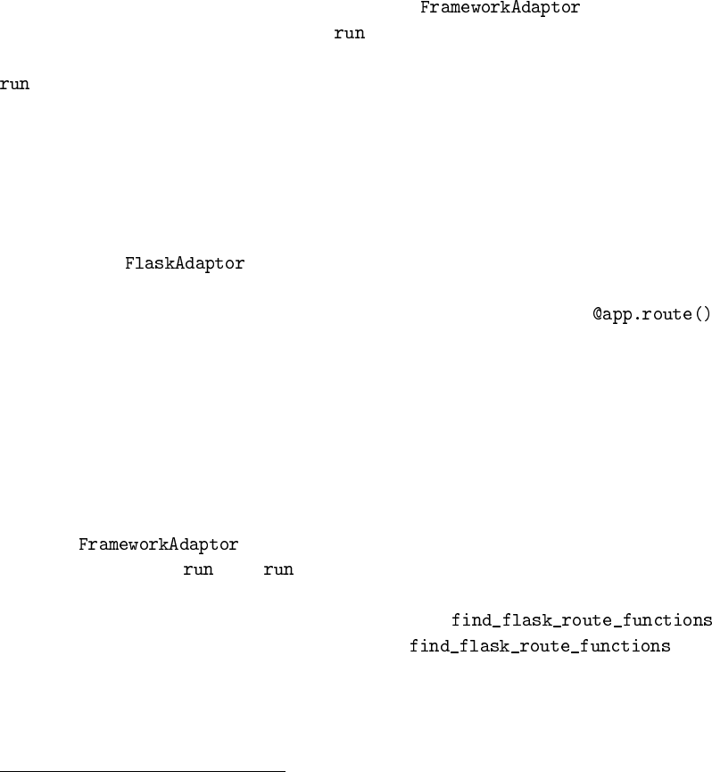
56 Chapter 7. Implementation
7.4 Framework adaptor
Our goal of our tool is to target web application frameworks. As there exist differ-
ent frameworks and these are organised in different manners, we need to accom-
modate for these variations. The framework adaptor is purposed to accommodate
for different web application frameworks. The class is an ab-
stract class with an abstract method . It contains a list of CFGs where the
adaptor is expected to put the result of the adaptation. The implementation of
should include processing for all framework specific details that are needed in
order to get a correct model of the application. This adaptor can be implemented
for an arbitrary framework like Django or, in our case, Flask.
The Flask Adaptor In Flask all web pages are defined in a function with a deco-
rator. This function is never explicitly called in the source code, so a single traversal
by the CFG visitor of the file will not include all these methods in the resulting list
of CFGs. The was implemented for this purpose. The result of the
CFG visitor contains all functions found during the traversal. The Flask adaptor
goes through these and finds all functions that are defined with the
decorator, and adds it to the list of CFGs. This results in a list of CFGs that cover
all the code needed for analysing the application.
Implementing a custom adaptor The adaptor component is in place for making
it possible to adapt the analysis to any framework. This paragraph will describe
how such an implementation should be devised.
In Appendix C the implementation of the Flask adaptor is shown. This imple-
mentation will be used as a basis for this description. The adaptor inherits from
the class which contains an instance variable for a CFG list and
the abstract function . The function is the entry point to an adaptor.
In the Flask implementation the CFG list, which is initially populated with the
result of the CFG visitor, is iterated over and the
function is called on each.
2
The idea of the was
described in the previous paragraph. A similar consideration has to be made for
the framework in question and then implemented in a similar fashion.
After implementing a custom adaptor, PyT will be able to analyse any applica-
tion using this framework.
2
In our case there is always one CFG in this list, but other implementations might have more than
one.

7.5. Flexible analysis 57
7.5 Flexible analysis
As mentioned in the implementation overview, the fixed point analysis is imple-
mented so that the analysis can be changed. For our purposes the modified reaching
definitions analysis presented in Section 6.11 is sufficient – it provides the answers
we need to locate the security vulnerabilities in web applications.
However, one could imagine improving PyT by utilising other analyses that
could help identify the vulnerabilities. In such a case PyT has been implemented
so it can be easily expanded with another analysis. The liveness analysis presented
in Schwartzbach [25, p. 19] has been implemented in order to exemplify the process
of implementing new analyses. This process will be explained in the following.
7.5.1 Implementing Liveness
The complete implementation is presented in Appendix D. The implementation
corresponds to the definition presented in Schwartzbach [25, p. 20]. The
class inherits from which contains logic for annotating the
CFG with extra information. In the case of the liveness analysis we need infor-
mation about the of each node. The deduction of these are defined as a
visitor which visits an AST node and finds the variables as defined
in Schwartzbach [25].
contains the constraints of the liveness analysis defined in
, which is shown in Listing 7.5. This method is used by the fixed
point analysis to apply the constraints on each node. This method uses a helper
which corresponds to the JOIN function in Schwartzbach [25], and the vari-
ables found by .
24
25
26
27
28
29
30
31
32
33
34
35
36
37
38
39
40
41

58 Chapter 7. Implementation
42
43
44
45
46
47
48
49
50
51
Listing 7.5: Implementation of liveness analysis -
With this implementation the PyT fixed point algorithm implementation can
perform liveness analysis on an arbitrary piece of python source code. The PyT
vulnerability checker could likewise be expanded with any analysis that could aid
the detection of security vulnerabilities.
7.6 Vulnerabilities
This module uses the result of the fixed-point analysis to detect vulnerabilities in
the application. First it is needed to determine which flows are dangerous. Then
taint analysis can be employed, and the resulting vulnerabilities will be recorded
and displayed in a readable manner to the developer.
7.6.1 Taint Analysis
In order to find dangerous flows in a program we need to know what expressions
introduce user input and what expressions may not receive input. We also need
to be able to detect when the program actually makes such input harmless. The
theoretical background for this was discussed in Section 6.10
1
2
3
Listing 7.6: A simple vulnerable program
The program in Listing 7.6 is vulnerable to a user executing arbitrary code.
is a source and is a sink. The result of is being handed
over to without any sanitisation. Imagine this program being served on a
server which also contains confidential information. An attacker would possibly
be able to retrieve this confidential information from the server.

7.6. Vulnerabilities 59
7.6.2 Sources, Sinks and Sanitisers in Flask
Flask is a web framework, so it uses some different means of user input than the
method. This section will cover a selection of these in order to have a basis
for performing an analysis of a Flask application.
Sources In Section 4.1 the object was introduced. This object is used to
access the input provided by the user through interaction with the page.
Query parameters Query parameters submitted to the URL of the format
’domain.com?query=parameter’ can be accessed with the
method. This method takes the key to retrieve a value from and a de-
fault value as parameters. If this methods returns a value that is different from the
default, it is potentially dangerous.
Form content Input submitted through form fields can be accessed with the
attribute. This attribute is a dictionary that maps a form field
to its value. Values retrieved from this dictionary are potentially dangerous.
Sinks User input can arrive at a wealth of methods which can be regarded as
a sink. We explored three vulnerabilities in Chapter 5 which we would like to
be able to detect. The following is the sinks that can possibly enable the chosen
vulnerabilities. These are obviously only a small selection of all possible sinks.
Homemade templates When utilising the template engine of Flask many se-
curity concerns are ruled out. An eager developer that is too impatient to read
the documentation for Jinja2 may resort to a solution that works, but is subpar re-
garding security. One example of this could be to use
instead of the template engine. The developer creates his own template format,
and replaces placeholders with user input. It works, but if the input does not get
sanitised, the user can inject javascript into the page, see Section 5.2.
The input passed to can be sanitised using the class
provided by Flask. is used to represent HTML markup and marks them
as being safe. It contains an function that escapes HTML tags and thereby
sanitises the input. Manipulating a markup object with string interpolation also
escapes all values. An example of escaping user input can be seen on Listing 7.7
where the method is used to sanitise the input before inserting it
with the method.
1
2
3

60 Chapter 7. Implementation
4
5
6
Listing 7.7: An example of escaping user input
Database access The recommended way to work with a database in Flask is
by using a package called SQLAlchemy[29, 30]. This package gives the developer
the option to setup and/or communicate with a database. In the following two ex-
amples of SQL injection, described in Section 5.1, will be presented. The complete
source code of the web application can be found in Listing A.1. The examples both
print out the result of the SQL queries to the console. In a real application there
would be some web interface where it is presented to the user.
The first example, Listing 7.8, shows that the address “/raw” takes a parameter
called . This parameter is then executed directly on the database. The result
is printed to the console. The problem here is that the user is able to execute every
query he wants. But SQLAlchemy prevents from executing several SQL commands
and from changing the database by for example deleting all of it.
1
2
3
4
5
6
Listing 7.8: An example of executing a raw sql query without sanitising.
The second example, Listing 7.9, shows how the parameter of the filter function
is not sanitised. The address “/filter” takes a parameter, , as input. This
is used directly in a filter function on the database. If the value of the
is “2 or 1 = 1” the filter function will return all users because the always
evaluates to true.
1
2
3
4
5
6
7
8
9
Listing 7.9: An example of inserting a raw sql parameter without sanitising it.

7.6. Vulnerabilities 61
Filesystem access Files can be sent to the client with the
method. This method takes a file from the filesystem and sends it to the user. If the
filename parameter is set by user input, the user can possibly traverse the filesys-
tem of the server, see Section 5.3. This can be sanitised by disallowing the use of
’..’ in the variable passed to the filename parameter.
7.6.3 Trigger Word Definition
A definition file is provided that contains sources, sinks and sanitisers which are
used to find vulnerabilities in the source code. A simple text file with two keywords
is used for this purpose. The keywords “sources:” and “sinks:” are used to indicate
the content of the section. Each source or sink is written on a separate line. A sink
can have a number of sanitisers attached written with as a comma separated list
after an arrow (“ ”). Sinks, sources and sanitisers are called trigger words, and
the definition file is called a trigger word file, and an example can be seen in
Listing 7.10. The defintion file used by PyT can be found in Appendix E.
1 s ource s :
2 source_1
3 source_2 (
4
5 sinks :
6 sink _1 [
7 sink _2 −> s a n i t i s e r _ 1
8 sink _3 −> s a n i t i s e r _ 1 , s a n i t i s e r _ 2 , s a n i t i s e r _ 3
Listing 7.10: How the trigger word file should be defined.
The words trigger a source if the trigger word is a substring of the node. This
means that the words have to be chosen carefully. Because of this, “function” and
“function(” can give different results Choosing the right one is therefore crucial.
This can appear too simple, but it gives more flexibility to define trigger words
that are either functions, indexes or have other characteristics without having an
elaborate but restrictive syntax for this.
7.6.4 Finding and Logging Vulnerabilities
After parsing the file all potential vulnerabilities are found and saved in a log. The
concept of finding vulnerabilities was described in Section 6.12. Vulnerabilities are
found by first identifying all nodes which contain a trigger word. All sources are
then checked if their constraint contain a source, and i that is the case, if a sanitiser
is in between the two. These cases are then logged to the vulnerability log. A
is an object which consists of a source and a sink CFG node, and
which words triggered the detection of these. A source and a sink have attached

62 Chapter 7. Implementation
a line number to them, this line number tells where they are located in the source
code. This information is used to make it as easy as possible for the developer to
find and determine whether the vulnerability found is harmful. An example of a
vulnerability log can be found in Listing 7.11. The output shown is after running
PyT on Listing 5.4. The vulnerability is reported by showing details of both source
and sink, with the relevant trigger word and the line number in the source code.
This should enable the developer to either fix the vulnerability or assess it as being
safe.
1 1 v u l n e r a b i l i t y found :
2 V u l n e r a b i l i t y 1 :
3 F i l e : example/vulnera ble _code/XSS . py
4 > User input at l i n e 6 , t r i g g e r word " get ( " :
5 param = r e q u e s t . args . g et ( ’ param ’ , ’ not s e t ’ )
6 Reassigned in :
7 F i l e : example/vulnerable_code/XSS . py
8 > Line 1 0 : ret_make_response = resp
9 F i l e : example/vulnera ble _code/XSS . py
10 > reach es l i n e 9 , t r i g g e r word " re p l a c e ( " :
11 resp = make_response ( html . re p l a c e ( ’ { { param } } ’ ,
param ) )
Listing 7.11: An example of how the vulnerability log looks after it found one vulnerability.
7.7 PyT
This section contains a description of how to use PyT. PyT is a command line tool
which requires one argument, the path of the file that should be analysed, and
several optional arguments. These are described below.
7.7.1 Positional Arguments
PyT requires one positional argument, , which is the path of the file which
should be analysed. If the file is a part of a project the folder in which the file is
in is used as root. To specify another root one can use the optional argument
explained below in Section 7.7.2.
7.7.2 Optional Arguments
This section contains a brief description of the optional arguments of PyT.
Project Root The project root argument is used for specifying the root of the
project when the filepath given is not in the root folder of the project.

7.7. PyT 63
Draw CFG This argument is useful to visualise a CFG. It outputs a PDF file that
contains a graph like the one on Figure 6.2.
Output Filename This argument can be used to specify the output name of the
file that is generated when using the or the argu-
ment.
Print This outputs the CFG to the standard output in simple representation. This
prints all labels of each node in the CFG.
Verbose Print The same as the print argument but more verbose. This means
that all information a node contains is send to the output.
Trigger Word File This argument is used for specifying a trigger word file which
is a file as defined in Section 7.6. This is optional as per default the Flask trigger
word file that comes with PyT.
Log Level This argument is used for setting the log level of the logger that is used.
The log level can be changed to the following levels, highest level first: CRITICAL,
ERROR, WARNING, INFO, DEBUG or NOTSET. Setting the log level will result
in the log containing messages from the chosen level and the levels above. The
default log level is and the logger writes the output of the logging to a
text file “logger.log”.
Adaptor This argument is used for specifying a framework adaptor. Per default
PyT uses the Flask adaptor which comes with it, see Section 7.4.
Create Database Creates a script that creates two database tables and inserts all
CFG nodes and all vulnerabilities. This feature is not tested due to time constraints.
Help This options shows a short overview of the available arguments and their
meaning. On Figure 7.4 the output of running PyT with this argument is depicted.
7.7.3 Command Line Argument Summary
Figure 7.5 shows a quick overview of the arguments of PyT and the corresponding
flags to use when running the tool.

64 Chapter 7. Implementation
Figure 7.4: An overview of PyT and its arguments.
Argument Description
Specify path of file to analyse.
Specify project root.
Draw CFG and output as a PDF file.
Name of the file that is output.
Prints a CFG with simple information about the nodes.
Same as print but with all information about the nodes.
Specify a trigger word file.
Set a log level.
Chose an adaptor.
Create a sql file of the CFG.
Figure 7.5: PyTs arguments.

7.8. Testing 65
7.8 Testing
During the development of the application we have had great success working test
oriented. In particular when developing the conversion from abstract syntax tree to
control flow graph, testing has been invaluable. The abstract nature of the syntax
tree together with the many possibilities of python yield a huge number of cases
for each construct, and the edges have to be just right in every one of them.
When developing all these fragments of the complete grammar, we need to be
sure that our previous work still works as intended. To help us be sure that all
our assumptions and implementations hold we have utilised unit testing a great
deal. The following will mention some of the issues where testing has helped the
process.
Cases An example of a construct which has many different cases is the con-
trol structure, which has variants with and statements. The abstract
syntax node contains an orelse reference which can either be another , represent-
ing an elif clause, or a list of statements, representing the body of an clause.
In addition an can have many different expressions in its test clause. These
expressions are often logic expressions but can also be nameconstants, function
calls, lambdas and even a list. To illustrate the three different cases three abstract
directed graphs have been made.
• The graph for a single statement can be seen on the left on Figure 7.6.
• The graph for an and an statement can be seen on the right on
Figure 7.6.
• The graph for an , and else statement can be seen on Figure 7.7
Note: On Figure 7.6 and Figure 7.7, expr is an expression and stmt* is a list of
statements.
When the basic cases of the is implemented we also need to know that
statements inside the body of an statement works properly. When that works
we need to consider how to handle , and statements inside the
.
Testing has greatly helped when exploring and developing these cases, because
they explicitly run each case every time the test is run. This assures that a change
fixing one case did not break another case.
Complex features The development of python is still ongoing which results in
periodic changes to both the grammar and the semantics of the language. Contin-
uously adding features from both the object oriented and the functional paradigm

66 Chapter 7. Implementation
if
test body orelse
expr stmt* [ ]
if
test body orelse
expr stmt* stmt*
Figure 7.6: Abstract graph showing the nodes in the abstract syntax tree for a single statement on
the left and an and statement on the right
if
test body orelse
expr stmt* if
test body orelse
expr stmt* stmt*
Figure 7.7: Abstract graph showing the nodes in the abstract syntax tree for an , and
statement

7.9. Limitations 67
results in more possibilities but also a more complex internal structure. This is
evident when attempting to generate control flow graphs from the abstract syntax.
One example is that you can assign a list to a tuple, and python will unpack and
assign the items of the list to the corresponding items of the tuple. This is possible
using the -operator. An example is show on Listing 7.12, where x is assigned the
value 4 and the tuple y is overwritten with the list [5, 6].
1
2
3
Listing 7.12: Tuple unpacking
Generating the control flow graph for expressions like these have given a lot of
insight into python, but it has also been a challenge to represent them properly in
the control flow graph. Also here testing has provided useful for keeping track of
the parts involved. The example consists of assignments, a tuple, the star operator
and a list in order to show off one concept. All the concepts both need to work
individually and together, and tests have helped ensuring this.
Dynamic types Python is a dynamic language which can be unforgiving to de-
bug. A wrong type returned from a function produces an error in a function
somewhere else. That can result in a big stack trace which can be hard to follow.
When developing with tests a catalogue of small tests are naturally developed.
When introducing an error that breaks more than just the construct at hand, test
have helped pinpointing the real cause of the error. This has sometimes lead to
insight that either helped us understand why our implementation was wrong, or
why what we expected was not the real outcome.
Integration test At last some integration tests were added to ensure that PyT
produces the right output for each vulnerability example described in Chapter 5.
This helped the process of implementing the vulnerability detection, by pointing
out when the detected vulnerabilities changed.
7.9 Limitations
This section will list the limitations that the implementation of PyT has.
7.9.1 Dynamic Features
The following dynamic features are not supported meaning that the right flow of
the source code is not captured and therefore is not taken into account in the anal-
ysis. PyT does not support the built in functions and . These functions

68 Chapter 7. Implementation
take a string as input which are executed as Python code. This means that the con-
tent of this string cannot be evaluated statically, and PyT cannot anticipate what
will happen.
PyT does also not support monkey patching. Monkey patching is used to re-
place functions in order to manipulate modules or classes. This is powerful but
also difficult to capture.
Not supporting the above dynamic features means that taint can be introduced
without PyT noticing. One way to fix this is to overtaint by just tainting all nodes
containing and for instance.
7.9.2 Decorators
Decorators are used to transform a function into another function. Flask uses this
to register functions that should be accessible as a webpage. In practice a decora-
tor is implemented as a class or a function that contains a transformation function
that returns the transformed function. When a function definition is decorated,
the transformed function will be used instead. An example was provided in Sec-
tion 3.1.6.
The current implementation does not perform this decoration process. A dec-
orated definition is not transformed, and the decorator is stored. This means that
some details may be lost. Some transformations may introduce taint, which will
not be caught by PyT.
A correct implementation of decorators will be very similar to that of a function
call, but there will be some considerations on how to capture the transformed
function correctly.
7.9.3 Libraries
The import handling does its best to find the implementation of functions called
throughout the program, but it can only find the implementation of functions
where the source code is available. This may be limiting the analysis, but having
to traverse all library code will be a major task. Fixing this requires considerations
of when it is worth doing, and when it is just increasing running time, without
adding value.
7.9.4 Language Constructs
This section contains a list of language constructs that were not implemented due
to time constraints and were not deemed important as most of them were not faced
in the projects we ran as input. Language constructs not implemented:
• Async - used for asynchronous programming.[31]
• Decorators - used for function transformations, explained in Section 3.1.6.
7.9. Limitations 69
• Try - used for catching exceptions.[32]
• Delete - a statement to delete a name.[33]
• Assert - a statement that can be used to insert debugging assertions into a
program.[34]
• Global - a statement that declares a name global so that one can access global
names from other scopes.[35]
• Yield - used in generator functions to “return” one item at a time.[36]
• Starred - used for unpacking (only partially implemented).[37]
Chapter 8
Discussion
This chapter contains an evaluation of PyT, reflections and future works.
8.1 Evaluation
This section will contain an evaluation of PyT. First the vulnerabilities described in
Chapter 5 will be run and serve as proof that the tool catches these vulnerabilities.
Thereafter PyT will be run on real projects and the performance of the tool will be
evaluated.
8.1.1 Detecting Manufactured Vulnerabilities
In Chapter 5 we presented four implementation mistakes that would leave a web
application vulnerable. In this section PyT will be run on the presented examples
to see if they are being detected as hoped.
SQL injection The first example was the SQL injection which can be found in
Appendix A.1. Here we expect to find the two vulnerabilities presented in Sec-
tion 5.1.1, the naive execution of the query parameter and the unescaped filter.
As seen on Figure 8.1 we get a report with two vulnerabilities. The first one
detected is the filtering vulnerability. PyT tells us that the trigger word ’get’ was
found in line 33, which then reached line 36 where the trigger word ’filter’ marked
it as a sink.
The second one is the naive implementation of the database query. Here the
vulnerability is reported to begin at line 26 where the trigger word ’get’ pointed
out a sink. This sink then reaches line 27 where the trigger word ’execute’ indicates
a sink.
Both vulnerabilities were thus able to be found by PyT.
71

72 Chapter 8. Discussion
Figure 8.1: Running PyT on the SQL injection example
Command injection The next example was the command injection which can be
found in Appendix A.2. Here we expect to find the one vulnerability presented in
Section 5.1.2 where the content of the form field reaches the subprocess call.
The execution of PyT on the example can be seen on Figure 8.2. PyT reports
one vulnerability being present in the application. A source is found on line 15
with the trigger word ’form’, which reaches a sink in line 18 marked because of
the trigger word ’subprocess.call’. In this case the source was assigned to a new
variable in line 16 to make up the complete command to be run. This is shown by
PyT as to provide information to the developer of how the tainted value did flow
through the code.
Cross site scripting The next vulnerability presented was the cross site scripting
attack described in Section 5.2. The code can be found in Appendix A.3.
The execution of PyT on the example can be seen on Figure 8.3. Here a source
is found in line 6 with the trigger word ’get’, which reaches the sink in line 9 with
the trigger word ’replace’. Notice that the vulnerability reports a reassignment in
line 10 which is irrelevant to the vulnerability because it happens after the sink.
Also notice that the reported line looks different than the source line because of
the CFG representation of a return node. This can potentially be confusing for the
user of PyT.
Sanitised cross site scripting example As mentioned in Section 6.12 some
vulnerabilities can be sanitised by special functions, making the dangerous code

8.1. Evaluation 73
Figure 8.2: Running PyT on the command injection example
Figure 8.3: Running PyT on the XSS example

74 Chapter 8. Discussion
Figure 8.4: Running PyT on the sanitised XSS example
Figure 8.5: Running PyT on the Path traversal example
harmless. Running PyT on the sanitised version presented in Listing 6.3 results in
the output presented in Figure 8.4
Here the vulnerability is found as in the above, but it concludes the vulnerabil-
ity report by adding that it is potentially sanitised by the ’escape’ function.
Path traversal The final vulnerability presented was the path traversal. The code
can be found in Appendix A.4. In this example we expect to find the vulnerability
presented in Section 5.3.
The execution of PyT on the example is shown in Figure 8.5. Here the report
shows one vulnerability, starting with a sink found in line 8 with the trigger word
’get’. This source then reaches the sink in line 11 which is detected by the trigger
word ’send_file’.

8.2. Reflections 75
Project Vulnerabilities
brightonpy.org[38] 0
flask-pastebin[39] 0
flask_heroku[40] 0
guacamole[41] 0
flamejam[42] 0
microblog[43] 0
flaskbb[44] undecided
Figure 8.6: Results.
8.1.2 Detecting Vulnerabilities in Real Projects
Six open source projects were tested with PyT, for evaluation its performance on
realistic inputs. A table with the results can be seen on Figure 8.6.
As one can see on the table, no vulnerabilities were found and there were even
one project where PyT did not terminate. This shows that PyT can be used for real
projects
Flaskbb Flaskbb did not terminate in a reasonable amount of time, and the run
was manually stopped. Upon further inspection it turns out to be due to the
amount of nodes being created. 432855 nodes were created, just in the main control
flow graph. This huge amount of nodes makes the analysis takes up much time
and space.
8.2 Reflections
This chapter will reflect on PyT and the experiences we have had during the de-
velopment of the tool.
8.2.1 Are Frameworks like Flask Good for Web Security?
In the beginning of the project period we had an idea of making a tool that could
find security flaws in web applications. We were well aware that vulnerabilities
would not be in an abundance. Even when looking at lists of well known vulner-
abilities, these were hard to apply to Flask applications. Flask takes care of a lot
without the user even having to think about it.
We therefore had to resort to the vulnerabilities we presented in Chapter 5.
These vulnerabilities are still dangerous, but could be unlikely to be found in the
wild. (Maybe with the exception of the command injection vulnerability. This may
actually be valid for some cases.)
76 Chapter 8. Discussion
Our experience with the Flask framework is therefore an indication that frame-
works like Flask definitely help security of web applications.
8.3 Future Works
This section contains a number of subjects which can be improved upon and
worked on in the future.
8.3.1 Better Trigger Word Definitions
Finding sources and sinks was a feature where the literature was sparse. Plenty of
papers use the terms, but no one described a clever way to find them. We therefore
devised our own system.
The implemented system uses a text file with the trigger words written in a
very simple syntax. The labels of CFG nodes are compared with the trigger words,
and if they contain one, they are marked as being either a source, a sink or a
sanitiser. Using this simple implementation we ran into problems like finding the
trigger word in variable names. The quick solution was to add a ’(’ to the trigger
word, which fixed that single problem.
In further development the whole trigger word system should be reconsidered.
The definition should be more sophisticated, and the comparison should be more
intelligent than just comparing in the label.
8.3.2 More Vulnerability Definitions
One of the reasons that our evaluation found no vulnerabilities in real applications
(see Section 8.1), is the small number of vulnerabilities PyT looks for. The used trig-
ger word definition file only finds those particular vulnerabilities that was found in
the beginning of the project. In order to make PyT really useful, this trigger word
definition should be expanded, not only with new vulnerabilities, but also with
variants of the vulnerabilities already being searched for. The two SQL injection
attacks presented in Section 5.1.1 is one example of a vulnerabilities where variants
of the same vulnerability exists. It is imaginable that many vulnerabilities exists in
a number of variants that all need to be defined by trigger words.
8.3.3 More Efficient Fixed-point Algorithm
In this project efficiency has not been a priority, and for the most part is has not
been a problem. In the evaluation performed on real projects, described in Sec-
tion 8.1.2, this suddenly became a hurdle. It turns out that big projects produce
CFGs that are so large that PyT simply does not terminate in a realistic amount
of time. It would therefore be a natural next step to attempt to improve this in-
8.3. Future Works 77
efficiency. As mentioned in Section 6.8 this project has not spent time examining
alternative implementations of the fixed-point algorithm. One suggestion would
therefore be to attempt to implement the improved version of the algorithm, in
order to get a faster analysis.
8.3.4 Expanding PyT with Other Analyses
As discussed in Section 7.5, PyT has been implemented in a flexible way, so that
any analysis can be implemented. This means that it is possible to expand the
analysis with supporting analyses. The implemented example, liveness analysis,
could be used to determine if a found vulnerability is in a piece of dead code. If this
is the case, the developer might not be interested in this particular vulnerability.
The danger of not displaying vulnerabilities in dead code is of course that this code
may become live at any time, and then the vulnerability is suddenly dangerous.
There could therefore be a optional command line flag that filters out dead code,
based on the liveness analysis.
Other analyses could also prove helpful in the detection of vulnerabilities.
8.3.5 Support More Frameworks
This project has only looked into the Flask web framework. In order to make
PyT even more useful, more frameworks should be supported. As mentioned in
Section 2.3, Django is a very popular framework. Implementing support for Django
could greatly increase the number of applications that PyT is able to analyse.
Implementing another framework requires a new adaptor. The process of writ-
ing a new framework adaptor was described in Section 7.4.
Chapter 9
Conclusion
This report engaged in creating a tool for detecting security flaws in Python web
applications. Firstly, the background for the project was examined, including the
Python programming language and the Flask web framework. We then proceeded
to manufacture some Flask applications with vulnerabilities. The resulting appli-
cations would then be used to check if the tool was able to detect them.
The theory needed to build such a tool was then described. The theory includes
control flow analysis, the monotone framework and taint analysis.
The tool PyT was then implemented with the aim of being flexible. PyT is
specialised to find vulnerabilities in Flask using a modified reaching definitions
analysis, but it is the intention that both aspects can be expanded on. It is thereby
possible to implement support for Django or use other analyses, without having to
make major changes.
At last PyT was evaluated. PyT was able to find all the manufactured vulnera-
bilities. It was also able to run on open source Flask projects and did not find any
vulnerabilities in these.
79

Appendix A
Vulnerability implementations
A.1 SQL injection
1
2
3
4
5
6
7
8
9
10
11
12
13
14
15
16
17
18
19
20
21
22
23
24
25
26
27
28
81

82 Appendix A. Vulnerability implementations
29
30
31
32
33
34
35
36
37
38
39
40
41
42
Listing A.1: SQL injection examples, using Flask and SQLAlchemy.
A.2 Command Injection
1
2
3
4
5
6
7
8
9
10
11
12
13
14
15
16
17
18
19
20
21
22
23
24
25

A.3. XSS 83
26
27
28
29
30
31
32
33
34
35
Listing A.2: Command injection example, using Flask.
A.3 XSS
1
2
3
4
5
6
7
8
9
10
11
12
13
14
15
A.4 Path Traversal
1
2
3
4
5
6
7
8
9
10

84 Appendix A. Vulnerability implementations
11
12
13
14
15

Appendix B
The Abstract Syntax of Python
The following shows the complete abstract syntax of the python programming
language. It is taken directly from Abstract Syntax of Python [45].
1 −− ASDL’ s s i x b u i l t i n types ar e i d e n t i f i e r , int , st r i n g ,
bytes , o bj e ct , s i n g l e t o n
2
3 module Python
4 {
5 mod = Module ( stmt ∗ body )
6 | I n t e r a c t i v e ( stmt ∗ body )
7 | Expression ( expr body )
8
9 −− not r e a l l y an ac t u a l node but u sef u l in Jython ’ s
typesystem .
10 | Su i t e ( stmt ∗ body )
11
12 stmt = FunctionDef ( i d e n t i f i e r name , arguments args ,
13 stmt ∗ body , expr ∗ d e c o r a t o r _ l i s t , expr
? re t u rn s )
14 | AsyncFunctionDef ( i d e n t i f i e r name , arguments args ,
15 stmt ∗ body , expr ∗ d e c o r a t o r _ l i s t
, expr ? r e t ur n s )
16
17 | ClassDef ( i d e n t i f i e r name ,
18 expr ∗ bases ,
19 keyword∗ keywords ,
20 stmt ∗ body ,
21 expr ∗ d e c o r a t o r _ l i s t )
22 | Return ( expr ? value )
85

86 Appendix B. The Abstract Syntax of Python
23
24 | Dele te ( expr ∗ t a r g e t s )
25 | Assign ( expr ∗ t a r g e t s , expr value )
26 | AugAssign ( expr tar g et , oper ator op , expr value )
27
28 −− use ’ orel s e ’ because e l s e i s a keyword i n t a r g e t
languages
29 | For ( expr t a r g e t , expr i t e r , stmt ∗ body , stmt ∗
o r e l s e )
30 | AsyncFor ( expr t a r g e t , expr i t e r , stmt ∗ body , stmt
∗ o r e l s e )
31 | While ( expr t e s t , stmt ∗ body , stmt ∗ o r e l s e )
32 | I f ( expr te s t , stmt ∗ body , stmt ∗ o r e l s e )
33 | With ( withitem∗ items , stmt ∗ body )
34 | AsyncWith ( withitem ∗ items , stmt ∗ body )
35
36 | Raise ( expr ? exc , expr ? cause )
37 | Try ( stmt ∗ body , e xcepthandler ∗ handlers , stmt ∗
or e l s e , stmt ∗ f i nalbody )
38 | Asser t ( expr t e s t , expr ? msg )
39
40 | Import ( a l i a s ∗ names )
41 | ImportFrom ( i d e n t i f i e r ? module , a l i a s ∗ names , i n t ?
l e v e l )
42
43 | Global ( i d e n t i f i e r ∗ names )
44 | Nonlocal ( i d e n t i f i e r ∗ names )
45 | Expr ( expr value )
46 | Pass | Break | Continue
47
48 −− XXX Jython w i l l be d i f f e r e n t
49 −− c o l _ o f f s e t i s the byte o f f s e t in the u t f8 s t r i n g
the pa r ser uses
50 a t t r i b u t e s ( i n t lineno , i n t c o l _ o f f s e t )
51
52 −− BoolOp ( ) can use l e f t & r i g h t ?
53 expr = BoolOp ( boolop op , expr ∗ va lues )
54 | BinOp ( expr l e f t , oper ator op , expr r i g h t )
55 | UnaryOp ( unaryop op , expr operand )
56 | Lambda ( arguments args , expr body )
57 | IfExp ( expr te s t , expr body , expr o r e l s e )

87
58 | Dict ( expr ∗ keys , expr ∗ values )
59 | S e t ( expr ∗ e l t s )
60 | ListComp ( expr el t , comprehension ∗ ge n erator s )
61 | SetComp ( expr el t , comprehension ∗ ge nerator s )
62 | DictComp ( expr key , expr value , comprehension∗
gener a t o r s )
63 | GeneratorExp ( expr el t , comprehension ∗ ge nerato r s )
64 −− the grammar c o n s t r a i n s where y i e l d e x p r e s s ions
can occur
65 | Await ( expr value )
66 | Yiel d ( expr ? value )
67 | YieldFrom ( expr value )
68 −− need sequences f o r compare to di s t i n g u i s h between
69 −− x < 4 < 3 and ( x < 4 ) < 3
70 | Compare ( expr l e f t , cmpop∗ ops , expr ∗ comparators )
71 | C all ( expr func , expr ∗ args , keyword∗ keywords )
72 | Num( o b j e c t n ) −− a number as a PyObject .
73 | S t r ( s t r i n g s ) −− need to s p e c i f y raw , unicode , e t c
?
74 | Bytes ( bytes s )
75 | NameConstant ( s i n g l e t o n value )
76 | E l l i p s i s
77
78 −− the fo l lowing expression can appear in assignment
co n t e xt
79 | A t t r i b u t e ( expr value , i d e n t i f i e r a t t r ,
expr_c o n t ext c t x )
80 | S ub s c ri p t ( expr value , s l i c e s l i c e , e x p r _context
c t x )
81 | S tarr e d ( expr value , expr _ c o ntext ct x )
82 | Name( i d e n t i f i e r id , e x p r_context c t x )
83 | L i s t ( expr ∗ e l t s , e x pr_context c t x )
84 | Tuple ( expr ∗ e l t s , e xpr_conte x t c tx )
85
86 −− c o l _ o f f s e t i s the byte o f f s e t in the ut f 8 s t r i n g
the pa r ser uses
87 a t t r i b u t e s ( i n t lineno , i n t c o l _ o f f s e t )
88
89 expr_c o n t ext = Load | St o r e | Del | AugLoad | AugStore |
Param
90

88 Appendix B. The Abstract Syntax of Python
91 s l i c e = S l i c e ( expr ? lower , expr ? upper , expr ? step )
92 | E x t S l i c e ( s l i c e ∗ dims )
93 | Index ( expr value )
94
95 boolop = And | Or
96
97 oper ator = Add | Sub | Mult | MatMult | Div | Mod | Pow |
L S h i f t
98 | R Sh i ft | BitOr | BitXor | BitAnd |
FloorDiv
99
100 unaryop = I n v e r t | Not | UAdd | USub
101
102 cmpop = Eq | NotEq | Lt | LtE | Gt | GtE | I s | IsNot |
In | NotIn
103
104 comprehension = ( expr tar g e t , expr i t e r , expr ∗ i f s )
105
106 ex cept hand ler = ExceptHandler ( expr ? type , i d e n t i f i e r ?
name , stmt ∗ body )
107 a t t r i b u t e s ( i n t lineno , i n t c o l _ o f f s e t )
108
109 arguments = ( arg ∗ args , arg ? vararg , arg ∗ kwonlyargs ,
expr ∗ kw_defaults ,
110 arg ? kwarg , expr ∗ de f a u l t s )
111
112 arg = ( i d e n t i f i e r arg , expr ? ann otati on )
113 a t t r i b u t e s ( i n t lineno , i n t c o l _ o f f s e t )
114
115 −− keyword arguments supplied to c a l l (NULL i d e n t i f i e r
f o r ∗∗kwargs )
116 keyword = ( i d e n t i f i e r ? arg , expr value )
117
118 −− import name with o p ti o n al ’ as ’ a l i a s .
119 a l i a s = ( i d e n t i f i e r name , i d e n t i f i e r ? asname )
120
121 withitem = ( expr context_e xpr , expr ? o pt i o na l _ v ar s )
122 }
Listing B.1: The abstract syntax of Python

Appendix C
Flask adaptor implementation
The following code listing presents the implementation of the adaptor that adapts
Flask projects to be analysed by PyT This is also the default adaptor used by the
PyT command line.
1
2
3
4
5
6
7
8
9
10
11
12
13
14
15
16
17
18
19
20
21
22
23
24
25
26
89

90 Appendix C. Flask adaptor implementation
27
28
29
30
31
32
33
34
35
36
37
38
39
40
41
42
43
44
45
46
47
48
49
50
51
52
53
54
55
56
57
58
59
60
61
62
63
64
65

91
66
67
Listing C.1: Implementation of the Flask adaptor

Appendix D
Implementation of the liveness anal-
ysis
1
2
3
4
5
6
7
8
9
10
11
12
13
14
15
16
17
18
19
20
21
22
23
24
25
26
27
28
93

94 Appendix D. Implementation of the liveness analysis
29
30
31
32
33
34
35
36
37
38
39
40
41
42
43
44
45
46
47
48
49
50
51
52
53
54
55
56
57
58
59
60
61
62
63
64
65
66
67
68
69
70
71
72
73
74
75

95
76
77
78
79
80
Listing D.1: Implementation of liveness analysis

Appendix E
Trigger word definition for flask
The following file is used as the default trigger definition file in PyT. It is tailored
for flask projects.
1
2
3
4
5
6
7
8
9
10
11
Listing E.1: Trigger word definition for flask projects
97

Bibliography
[1] Attackers have advantage in cyberspace, says cybersecurity expert.
. Accessed: 2016-04-13.
[2] How important is website security?
. Accessed: 2016-04-13.
[3] The OWASP Top Ten Project.
. Accessed: 2016-04-04.
[4] Juan José Conti and Alejandro Russo. “A taint mode for python via a li-
brary”. In: Information Security Technology for Applications. Springer, 2010, pp. 210–
222.
[5] The Rough Auditing Tool.
. Accessed: 2016-05-14.
[6] Levin Fritz. Balancing Cost and Precision of Approximate Type Inference in Python.
2011.
[7] Web Frameworks for Python. .
Accessed: 2016-05-17.
[8] Django. . Accessed: 2016-05-17.
[9] Avraham Leff and James T Rayfield. “Web-application development using
the model/view/controller design pattern”. In: Enterprise Distributed Object
Computing Conference, 2001. EDOC’01. Proceedings. Fifth IEEE International.
IEEE. 2001, pp. 118–127.
[10] Flask Web Application Framework. . Accessed: 2016-
04-11.
[11] Python 3.5.1 documentation. . Accessed: 2016-
04-08.
[12] Data structures in Python.
. Accessed: 2016-04-15.
[13] Mark Lutz. Learning python. " O’Reilly Media, Inc.", 2013.
99

100 Bibliography
[14] Is Python pass-by-reference or pass-by-value?
. Accessed: 2016-05-23.
[15] Defining Functions.
. Accessed: 2016-05-23.
[16] The Zen of Python. . Accessed:
2016-04-12.
[17] Functional programming in Python.
. Accessed: 2016-04-12.
[18] Flask Documentation. . Accessed: 2016-
04-11.
[19] SQLAlchemy - The Python SQL Toolkit.
. Accessed: 2016-04-12.
[20] OWASP Top 10 - 2013 - The Ten Most Critical Web Application Security Risks.
. Ac-
cessed: 2016-04-05.
[21] SQL injection in CWE. .
Accessed: 2016-04-05.
[22] Command injection in CWE.
. Accessed: 2016-04-05.
[23] Cross site scripting in CWE.
. Accessed: 2016-04-05.
[24] Path traversal in CWE. .
Accessed: 2016-04-05.
[25] Michael I Schwartzbach. “Lecture notes on static analysis”. In: Basic Research
in Computer Science, University of Aarhus, Denmark (2008).
[26] Edward J Schwartz, Thanassis Avgerinos, and David Brumley. “All you ever
wanted to know about dynamic taint analysis and forward symbolic execu-
tion (but might have been afraid to ask)”. In: Security and privacy (SP), 2010
IEEE symposium on. IEEE. 2010, pp. 317–331.
[27] - Abstract Syntax Trees. .
Accessed: 2016-04-15.
[28] John Vlissides, Richard Helm, Ralph Johnson, and Erich Gamma. “Design
patterns: Elements of reusable object-oriented software”. In: (1994).
[29] SQLAlchemy. . Accessed: 2016-05-2.
[30] SQLAlchemy Documentation. .
Accessed: 2016-04-12.

Bibliography 101
[31] asyncio - Asynchronous I/O, event loop, coroutines and tasks.
. Accessed: 2016-05-26.
[32] Errors and Exceptions. .
Accessed: 2016-05-26.
[33] The del statement.
. Accessed: 2016-05-26.
[34] The assert statement.
. Accessed: 2016-05-26.
[35] The global statement.
. Accessed: 2016-05-26.
[36] Unpakcing Argument Lists.
. Accessed: 2016-05-26.
[37] Unpakcing Argument Lists.
. Accessed: 2016-05-26.
[38] brightonpy.org. . Accessed:
2016-05-29.
[39] flask-pastebin. . Accessed:
2016-05-29.
[40] flask_heorku. . Accessed: 2016-
05-29.
[41] guacamole. . Accessed: 2016-05-
29.
[42] flamejam. .
Accessed: 2016-05-29.
[43] microblog. . Accessed:
2016-05-29.
[44] flaskbb. . Accessed: 2016-05-29.
[45] Abstract Syntax of Python.
. Accessed: 2016-05-17.
