Is resale needed in markets with refunds? Evidence from college football ticket sales

Vollmer, Drew

Working Paper

Is resale needed in markets with refunds? Evidence

from college football ticket sales

EAG Discussion Paper, No. EAG 22-2

Provided in Cooperation with:

Economic Analysis Group (EAG), Antitrust Division, United States Department of Justice

Suggested Citation: Vollmer, Drew (2022) : Is resale needed in markets with refunds? Evidence

from college football ticket sales, EAG Discussion Paper, No. EAG 22-2, U.S. Department of Justice,

Antitrust Division, Economic Analysis Group (EAG), Washington, DC

This Version is available at:

https://hdl.handle.net/10419/284002

Standard-Nutzungsbedingungen:

Die Dokumente auf EconStor dürfen zu eigenen wissenschaftlichen

Zwecken und zum Privatgebrauch gespeichert und kopiert werden.

Sie dürfen die Dokumente nicht für öffentliche oder kommerzielle

Zwecke vervielfältigen, öffentlich ausstellen, öffentlich zugänglich

machen, vertreiben oder anderweitig nutzen.

Sofern die Verfasser die Dokumente unter Open-Content-Lizenzen

(insbesondere CC-Lizenzen) zur Verfügung gestellt haben sollten,

gelten abweichend von diesen Nutzungsbedingungen die in der dort

genannten Lizenz gewährten Nutzungsrechte.

Documents in EconStor may be saved and copied for your personal

and scholarly purposes.

You are not to copy documents for public or commercial purposes, to

exhibit the documents publicly, to make them publicly available on the

internet, or to distribute or otherwise use the documents in public.

If the documents have been made available under an Open Content

Licence (especially Creative Commons Licences), you may exercise

further usage rights as specified in the indicated licence.

ECONOMIC ANALYSIS GROUP

DISCUSSION PAPER

Is Resale Needed in Markets with Refunds?

Evidence from College Football Ticket Sales

Drew Vollmer

EAG 22-2 December 2022

EAG Discussion Papers are the primary vehicle used to disseminate research from economists

in the Economic Analysis Group (EAG) of the Antitrust Division. These papers are intended

to inform interested individuals and institutions of EAG’s research program and to stimulate

comment and criticism on economic issues related to antitrust policy and regulation. The

Antitrust Division encourages independent research by its economists. The views expressed

herein are entirely those of the author and are not purported to reflect those of the United States

Department of Justice.

Information on the EAG research program and discussion paper series may be obtained from

Russell Pittman, Director of Economic Research, Economic Analysis Group, Antitrust

Division, U.S. Department of Justice, LSB 9004, Washington, DC 20530, or by e-mail at

russell.pittman@usdoj.gov. Comments on specific papers may be addressed directly to the

authors at the same mailing address or at their e-mail address.

Recent EAG Discussion Paper and EAG Competition Advocacy Paper titles are available

from the Social Science Research Network at www.ssrn.com. To obtain a complete list of

titles or to request single copies of individual papers, please write to Keonna Watson at

K e onna . Wa ts on@usdoj.gov or call (202) 307-1409. In addition, recent papers are now

available on the Department of Justice website at

http://www.justice.gov/atr/public/eag/discussion-papers.html.

Antitrust Division, U.S. Department of Justice. Email: Andrew.Vollmer@usdoj.gov.

Is Resale Needed in Markets with Refunds?

Evidence from College Football Ticket Sales

Drew Vollmer

∗

February 27, 2022

Abstract

When is resale valuable? And when can it be replaced with re-

funds? I study the performance of common reallocation mechanisms

in perishable goods markets with demand uncertainty. Using primary

and secondary market data on college football ticket sales, I design a

structural model to evaluate the performance of resale, partial refunds,

and a menu of refund contracts. In the model, consumers anticipate

shocks when making initial purchases. After shocks are realized, they

participate in an endogenous resale market. I ﬁnd that refunds are more

eﬃcient than resale, but that resale is better for sellers and consumers

than not reallocating.

∗

U.S. Department of Justice. Contact: drew.v[email protected]

The views expressed are those of the author and do not necessarily represent those of the

U.S. Department of Justice. I am grateful for helpful conversations with and comments from

Allan Collard-Wexler, James Roberts, Curtis Taylor, Bryan Bollinger, Jonathan Williams,

Daniel Xu, Juan Carlos Su`arez Serrato, Peter Newberry, and Matt Leisten. I also beneﬁted

from seminar and conference presentations at Duke, the SEAs, and the DC IO Day. I would

like to thank the university that provided its sales records for the project. All errors are

mine.

1 Introduction

Is resale valuable? The usual answer is yes, because it reallocates goods

to consumers with high values. For instance, a consumer might buy

a concert ticket, learn she cannot attend, and resell to someone who

can. But there are other methods of reallocating, like refunds, that

could reach the same result. With refunds, the consumer could return

the ticket to the box oﬃce for a partial refund, allowing the seller to

oﬀer the recovered ticket to someone else. In fact, many sellers, like air-

lines and hotels, oﬀer partial refunds instead of allowing resale. Would

society be better oﬀ if resale were replaced with refunds, or is resale

uniquely valuable? The question matters because reallocation is nec-

essary when consumers receive stochastic demand shocks after initial

purchases. They do so frequently: a consumer might make travel plans

in advance and then learn she has a schedule conﬂict, or she might buy

clothes online and then learn they do not ﬁt.

In this paper, I evaluate the most common reallocation mechanisms,

resale and refunds, in markets for perishable goods with demand un-

certainty. I use data on college football ticket sales to study the perfor-

mance of resale and two refund strategies, a partial refund and a menu

of state-dependent refund contracts. With a partial refund, consumers

who buy in advance can return the good for some money back; with

a menu of refunds, consumers who buy in advance can choose among

contracts that issue refunds in diﬀerent states of the world. Football

tickets are an ideal setting because consumers purchase in advance and

then receive diﬀerent demand shocks,

including schedule conﬂicts and

aggregate shocks like news about team performance.

After presenting examples in which each strategy can be most eﬃ-

cient, I assess their performance empirically with a structural model in

which consumers purchase football tickets over two periods. In the ﬁrst

period, consumers decide whether to buy season tickets based on ratio-

nal expectations of shocks and future resale prices. In the second period,

Sweeting (2012) uses sports tickets to study perishable goods. Event tickets have also

been used as a setting in Leslie and Sorensen (2014).

shocks are realized and consumers make ﬁnal purchase decisions. Con-

sumers who bought tickets in the ﬁrst period choose whether to attend

or resell; other consumers decide whether to acquire tickets in the pri-

mary or resale markets. The resale price clears the resale market in the

second period and thus depends on realized shocks. In counterfactual

experiments, I replace the resale market with refund policies.

The results suggest that refunds perform as well as resale and are

superior when consumers have heterogeneous preferences over an un-

certain state of the world. By quantifying the eﬀects of resale and

comparing it to refunds, the ﬁndings inform the design of aftermarkets

and government policies on resale rights.

The key diﬀerence between the strategies is that refunds are central-

ized in the primary market and resale is not. With refunds, consumers

can return their tickets to the primary seller, who puts the recovered

units back on sale. All transactions take place in the primary market at

the seller’s prices. But with resale, consumers can list their tickets on a

third-party resale platform, like StubHub, at prices they choose. Cen-

tralization is beneﬁcial because it reduces frictions and allows the seller

to oﬀer a menu of state-dependent refund contracts; it can be harmful

when primary market prices are suboptimal because of rigidities and

menu costs, unlike resale’s ﬂexible prices.

In numerical examples, I show that each strategy can be most eﬃ-

cient. Suppose that a sports team sells tickets in advance and cannot

change its prices.

Some consumers will purchase early, then learn they

have schedule conﬂicts and cannot attend. If the optimal price is un-

certain, price rigidities can cause partial refunds to perform badly. For

example, suppose the team’s star player is injured, causing consumer

values to fall. Consumers with conﬂicts will request a partial refund,

but the seller’s price will be too high to sell the recovered tickets after

the injury. Some tickets will go unused. Resale would perform better

because its prices are ﬂexible: resellers would lower prices after the in-

The strong assumption of complete rigidity holds in my setting, where prices are printed

on the tickets. Weaker rigidities have a similar eﬀect for other sellers, who do not adjust

prices to fully reﬂect changes in demand. As shown in Section 4, observed demand shifts

are empirically large.

jury so that all tickets are sold and used. But resale is less eﬃcient

when there is no need for price ﬂexibility because it introduces addi-

tional frictions. For example, some consumers may be unaware of the

resale market, or they may dislike browsing or distrust the platform.

The choice between partial refunds and resale depends on the relative

intensity of mispricing and frictions, which must be recovered in esti-

mation.

A separate force determines the value of state-dependent refund con-

tracts: whether diﬀerent consumers want the tickets in diﬀerent states

of the world. For instance, the consumers who value tickets the most

in a state where covid-19 disappears might not be the same as the

consumers who value them most in a state with widespread infection.

With a menu of refund contracts, the seller could target each group

with refunds that depend on the status of covid-19 or, more generally,

an observable state.

After estimating the model, I ﬁnd in counterfactual experiments

that the refund strategies are as eﬃcient as resale when there is no un-

certainty over states of the world. Total welfare is 0.5% higher with

refunds and consumer welfare is unchanged, but the seller does earn

2.1% more in proﬁt. The results are noteworthy because they suggest

that, even in a market with inﬂexible prices and aggregate shocks, resale

can be replaced. All parties beneﬁt from resale and refunds compared

to a market without reallocation: total welfare increases by 5.1%, con-

sumer welfare by 6.9%, and proﬁt by 2.8%. The changes are substantial

because only 8% of tickets are reallocated in the estimated model. In

counterfactuals with uncertainty over whether there will be a covid-19

vaccine, the menu of state-dependent refund contracts oﬀers marked

beneﬁts over resale, raising total welfare by 5.5%, consumer welfare by

8.8%, and proﬁt by 4.5%.

The analysis has broad implications for our understanding of af-

termarkets and resale. Evidence on the performance of reallocation

Refunds are optimal when primary market prices are ﬂexible, as for airlines and hotels.

A related source of uncertainty is if consumers have diﬀerent probabilities of having a

schedule conﬂict, studied in Lazarev (2013).

mechanisms, and of the factors that aﬀect them, is valuable for deter-

mining how to run aftermarkets. Yet there is little work on the matter.

This paper contributes by highlighting the forces that determine when

each strategy is eﬃcient and evaluating the strategies empirically. It

also contributes to our understanding of resale by quantifying its net

eﬀects. The eﬀects of resale on both sellers and society have been hotly

contested, with governments alternately restricting and protecting re-

sale of event tickets.

Similarly, some sellers prohibit resale while others

embrace it.

Some of the controversy is due to systematic underpric-

ing, which is not present in this setting, but the net eﬀect of resale

on proﬁt remains ambiguous in theory

and the beneﬁts for consumers

have rarely been measured. Additionally, the relevant class of perishable

goods is large, covering items like reservation goods (e.g. live events,

airlines, hotels, etc.) and seasonal goods (fashion). Online event ticket

sales alone exceeded $56bn in 2019 (Statista (2020)).

The application with state-dependent contracts is valuable because

it quantiﬁes the eﬀects of screening when consumers are heterogeneous,

which are frequently discussed in theory (Courty and Li, 2000) but

rarely measured empirically.

The empirical application to covid-19 is

relevant because of the return of mass gatherings despite uncertainty

over the future status of covid-19 and the resistance oﬀered by vaccina-

tion.

The analysis also oﬀers suggestive evidence on alternatives to re-

sale when there are rent-seeking brokers. Much of the resale literature

focuses on markets where brokers purchase underpriced tickets in the

primary market, as in Bhave and Budish (2017) and Leslie and Sorensen

(2014). In fact, Courty (2019) proposes a refund system to eliminate

Many states prohibit resale at prices above face value but have exempted internet sales

(Squire Patton Boggs LLP (2017)). Others forbid sellers from using non-transferrable tick-

ets, which are designed to prevent resale (Pender (2017)).

Musicians like the band U2 have prohibited resale for their concerts (Pender (2017)),

but many sports teams have sponsorship deals with platforms like StubHub and SeatGeek.

The key determinant in this setting is whether resale displaces primary market sales.

Resale is more proﬁtable when capacity constraints are tighter.

An exception is Lazarev (2013), who measures the eﬀects of screening airline passengers

who receive schedule conﬂicts at diﬀerent rates.

brokers similar to the one tested in this paper. Underpricing and bro-

kers are not signiﬁcant in this setting, but the performance of resale

relative to refunds provides suggestive evidence on brokers because bro-

kers magnify both the advantages and disadvantages of resale. Brokers

funnel more tickets through the resale market, leading to more price

ﬂexibility and frictions from resale. However, the predictions are not

deﬁnitive because estimated parameters and the initial allocation would

be diﬀerent with brokers. For example, resale frictions may be lower

with fewer tickets left in the primary market. Similarly, refunds may

perform worse with systematic underpricing because more tickets would

be rationed.

The most important feature of the model is the set of demand shocks

that aﬀect consumer values between the time of initial purchases and

the time of the game. The model includes three distinct shocks that are

common in other markets and salient in the market for football tickets.

The ﬁrst shock is purely idiosyncratic and can be interpreted as a

schedule conﬂict, which is common in markets for event tickets and

travel reservations. It causes some consumers who purchase early to

have low ﬁnal values, motivating reallocation. The second shock, a

common value shock, shifts all consumers’ values by the same amount

and can be interpreted as learning the quality of a good, like the skill of

a sports team or weather in a vacation destination. It makes the mean

valuation and optimal price after shocks unpredictable, boosting the

returns to resale and its ﬂexible prices. The third shock is a state of the

world that has a heterogeneous eﬀect on consumer values. The recession

state of a business cycle, for example, harshly aﬀects some consumers

but hardly aﬀects others. In the market for tickets, the states can be

interpreted as the future status of covid-19, which could ebb or continue

to pose a risk to the vaccinated. The estimation captures the associated

uncertainty using survey data on a similar shock, whether there will be

a covid-19 vaccine (assumed to be eﬀective) at the start of the season.

The survey was distributed in August 2020, when it was unclear if or when there would

be a vaccine. When the survey was distribtued, consumers were unlikely to be aware of the

possibility of breakthrough cases and the Delta variant had not yet been detected.

States of the world cause the eﬃcient allocation to vary with the state,

increasing the return to a menu of state-dependent refund contracts.

I assemble a broad data set to learn about the market and shocks.

The main data set consists of all primary and resale market ticket sales

for one football season at a large U.S. university, covering 30,000 pri-

mary market transactions and 5,500 resale transactions on StubHub.

The data demonstrate that advance sales and resale are features of the

market: 75% of tickets are sold months in advance and 6% of all tick-

ets are resold on StubHub. The second data set includes annual resale

prices for 76 college football teams from 2011–2019, which I gather

from SeatGeek, another online resale market. Resale prices vary signif-

icantly, often diﬀering from the sample average by 25% or more. The

ﬁnal source of data is a survey. In August 2020, I asked 500 consumers

(250 of whom were 50 or over) their willingness to pay for football tick-

ets in states with and without a covid-19 vaccine. Consumer reactions

to the state with no vaccine are heterogeneous: among consumers with

positive willingness to pay when there is a vaccine, almost a third would

pay the same amount with no vaccine while a ﬁfth would pay nothing.

I estimate the model in two stages. The key parameters in the ﬁrst

stage govern the demand shocks. The rate of idiosyncratic shocks is

identiﬁed by the frequency of observed resale in the ticket sales data.

The size of common value shocks, such as injuries and team perfor-

mance, is identiﬁed by year-to-year price variation in the SeatGeek data.

Heterogeneity in values between states with and without a vaccine is

captured by a distribution of value changes. The distribution is identi-

ﬁed by individual-level reports of changes in willingness to pay in the

survey.

The second stage uses structural simulations to estimate demand

and other remaining parameters. The simulations match observed to

simulated resale prices and primary market quantities. The compu-

tational challenge is ﬁnding a rational expectations equilibrium where

The NFL has oﬀered a similar refund contract where fans only receive a Super Bowl

ticket if their favorite team is in the game. More generally, the principle of contracting on

observed states is the basis for ﬁnancial derivatives.

There is resale on other sites, but StubHub is the largest resale service (Satariano (2015))

consumers correctly anticipate the distribution of resale prices.

The estimated model allows me to evaluate two core sets of coun-

terfactuals. In the ﬁrst, I consider a baseline model without states of

the world and compare resale to partial refunds. I also consider bench-

mark cases with no reallocation (neither resale nor refunds) and ﬂexible

prices (refunds with price adjustments after shocks). In the second set

of counterfactuals, the only uncertainty is over the state of the world

and I compare the performance of a menu of refunds to resale.

The remainder of the introduction discusses the relevant literature.

Section 2 presents numerical examples demonstrating how the prop-

erties of demand uncertainty aﬀect the seller’s optimal sales strategy.

Section 3 discusses the data sources used, and Section 4 presents de-

scriptive evidence. Section 5 develops a structural model of the market

and Section 6 details how it is estimated. Section 7 presents the coun-

terfactual experiments and their results. Section 8 concludes.

Related Literature. This paper contributes to several literatures, no-

tably those on resale and demand uncertainty. For the resale literature,

this paper provides estimates of how resale aﬀects proﬁt and welfare by

modeling a primary market and an endogenous resale market. Leslie

and Sorensen (2014) use a similar model combining primary and re-

sale markets to study whether resale increases welfare in the market

for concert tickets, but they do not consider proﬁt because tickets are

systematically underpriced in their sample. Tickets in my setting are

not underpriced and so I study both proﬁt and welfare. Sweeting (2012)

also studies the resale of event tickets, focusing on the use of dynamic

pricing in online resale markets. Lewis et al. (2019) investigate the ef-

fect of resale on demand for season tickets in professional baseball but

do not model how resale of season tickets aﬀects sales of other tickets.

The net eﬀects of resale on buyers and sellers are a traditional focus of

the theory literature on resale, including studies such as Courty (2003)

The menu of refunds is not mutually exclusive from other sales strategies when the full

refund depends on the state. Consumers who receive tickets in the realized state might

still receive idiosyncratic shocks, which leaves room for resale and partial refunds. I do not

consider idiosyncratic shocks to avoid testing combinations of the sales stratgies.

and Cui et al. (2014).

A separate literature considers resale of durable goods. With durable

goods, sellers compete against past vintages of their products, as in

Chen et al. (2013).

This paper also broadens the traditional focus on resale to con-

sider alternative methods of reallocation. Two recent studies, Cui et al.

(2014) and Cachon and Feldman (2018), have compared resale and re-

funds in theory, but neither involves empirics or aggregate shocks.

The current analysis also relates to studies of demand uncertainty

in which aggregate uncertainty aﬀects ﬁrms’ strategic choices, such as

Kalouptsidi (2014), Jeon (2020), and Collard-Wexler (2013). This paper

diﬀers by focusing on strategies ﬁrms can use to cope with uncertainty.

The emphasis is similar to studies of airline pricing with stochastic

demand, such as Lazarev (2013) and Williams (2020), where stochastic

consumer arrivals make dynamic pricing proﬁtable. In contrast, this

paper focuses on non-price strategies for reallocation.

2 Examples

In this section, I present examples illustrating how demand shocks aﬀect

each sales strategy. The examples show that each strategy can maximize

welfare and proﬁt, with the result depending on the relative strength of

the shocks.

The structure of the examples closely resembles the empirical model.

In each example, there are two periods and the seller has one ticket to

sell to two consumers. The seller can set diﬀerent prices for each period

but, like the seller in the data, it must commit to its menu at the start of

the ﬁrst period. Consumers are forward-looking and one arrives in each

period. Suppose that consumer i has value u

= ν

+ V − b

(ω), where

is consumer i’s preference for the ticket, V is a common component

to values shared by all consumers, and b

(ω) is consumer i’s individual-

speciﬁc response to state of the world ω.

Values are aﬀected by three potential shocks realized at the start of

the second period. The ﬁrst shock is purely idiosyncratic, like schedule

conﬂicts: each consumer i receives a shock with probability ψ. Draws

are independent and consumers who receive a shock have zero value.

The second shock changes the common value V , like injuries or team

performance. The third shock is a state of the world ω ∈ {ω

, ω

}, like

recessions or the status of covid-19, that aﬀects the b

(ω) term.

Suppose that resale incurs the friction s, so a resale purchase at

price p

earns utility u

− p

− s. (All resale takes place in the second

period.) The friction could be due to search costs or distaste for the

resale market. Furthermore, the resale market operator charges a mul-

tiplicative fee τ, so the buyer pays the fee-inclusive price p

while the

reseller receives (1 − τ)p

. The reseller makes a take-it-or-leave-it oﬀer

of p

in the examples, but the assumption is only used for simplicity.

Illustrations and a more detailed explanation of each equilibrium

can be found Appendix A.

Example 1: Idiosyncratic Shocks. Suppose that there are only idiosyn-

cratic shocks: ψ =

but V = 0 and b

(ω) = 0. The ﬁrst consumer,

Alice, arrives in the market in the ﬁrst period and prefers to buy early;

she has value ν

= 50 in period one, but it falls to ν

= 40 if she waits

to purchase until the second period. The second consumer, Bob, arrives

in period two with ν

= 40 and never receives an idiosyncratic shock.

The seller optimally oﬀers a partial refund r = 5 and sets p

= 41,

= 40.

Alice purchases the ticket in the ﬁrst period despite the risk

of a schedule conﬂict.

If Alice has a schedule conﬂict, she will return her ticket for a partial

refund; Bob then buys the ticket from the seller for p

= 40. Expected

proﬁt and total welfare equal 48, the highest possible value.

With resale, welfare would be lower because of frictions and proﬁt

would be lower because of frictions and fees. Suppose that τ =

and s = 1. In the second period, Alice would resell to Bob at price

With many agents, as in the empirical model, the TILI assumption is not necessary. I

use it here to simplify equilibrium with two agents.

The choice of r = 5 is optimal but not unique. The seller could produce the same

allocation and division of surplus by oﬀering any refund r such that Alice returns her ticket

if and only if she receives an idiosyncratic shock. For any such r, it can charge p

= 40 + ψr

but will pay ψr in expected refunds.

39 because of the resale friction, leading to lower total welfare of 47.8.

Alice only receives 35.10 after fees, so the seller can only charge her

35.10 when she has a conﬂict, leading to proﬁt of p

= 47.02.

Resale remains superior to not reallocating: total surplus and proﬁt

would be 40 without resale or refunds. However, resale is less valuable to

the seller when there are many tickets to sell and resale merely displaces

demand for tickets in the primary market.

Example 2: Idiosyncratic and Common Value Shocks. Resale can be

superior when ﬂexible prices are valuable, such as when there are com-

mon value shocks. Consider the same setting but suppose that the star

player is injured with probability

, leading to V = −20, and V = 0

otherwise.

If the seller oﬀers a partial refund, it will set r = 5, p

= 37, and

= 40.

As before, Alice purchases in the ﬁrst period. The key

diﬀerence is that Bob is unwilling to purchase at the seller’s optimal

price of p

= 40 after an injury. The seller’s rigid prices thus make

it possible that Alice will request a refund and Bob will not purchase,

causing the ticket to go to waste. Expected proﬁt and welfare equal 42.

But with resale, Alice could resell to Bob at both common values,

setting p

= 39 when V = 0 and p

= 19 when V = −20. Expected

total welfare rises to 42.8 and expected proﬁt to 42.12 because the ticket

is now reallocated and used when V is low.

The ﬁrst two examples illustrate the tradeoﬀ between resale’s price

ﬂexibility and its frictions. When price ﬂexibility is not valuable, as in

the ﬁrst example, partial refunds are superior because they avoid resale

frictions (and, for proﬁt, fees). But when price ﬂexibility is valuable,

as in the second example, resale can be eﬃcient and proﬁt-maximizing.

An empirical model is needed to determine which eﬀect dominates.

Example 3: States of the World. A menu of state-dependent contracts

is best when the eﬃcient allocation depends on the state of the world.

Suppose there are are no idiosyncratic or common value shocks, ψ = 0

For a general analysis, see Cui et al. (2014).

As before, the choice of r = 5 is optimal but not unique. The division of surplus is

again the same with other optimal selections of r.

and V = 0, but that there are two states, ω

with widespread vaccina-

tion or low caseloads and ω

with higher risk, and that each occurs with

probability

. The state is realized at the start of the second period.

Alice and Bob both arrive in the ﬁrst period, and the seller only makes

sales in the ﬁrst period. Alice’s value is ν

= 40 and does not respond

to the shock—she has b

(ω

) = 0. Bob has ν

= 50 but responds

harshly to the shock, b

(ω

) = 40.

If the seller oﬀered a single price, it would set p = 40 and sell to

Alice. But in state ω

, Alice would have the ticket when Bob has

a higher value. A single refund would not help because Alice would

return her ticket in both states.

With resale, Alice could resell to Bob

in the good state, but at the cost of fees and frictions.

A menu of state-dependent contracts would avoid fees and maximize

welfare and proﬁt. The seller could oﬀer a contract granting a full refund

in state ω

at price 50, which Bob would purchase, and another granting

a full refund in state ω

at price 40, which Alice would purchase. The

menu is valuable because Alice and Bob have heterogeneous reactions to

the realized state, making the consumer with the highest value diﬀerent

in each state. If there were no heterogeneity, then one consumer would

have the highest value in both states and the menu would add no value,

as in the ﬁrst two examples.

3 Data

The analysis relies on three data sets. The ﬁrst consists of ticket sales for

a single university, covering both the primary and resale markets. Ticket

sales are informative about demand for tickets and the extent of resale.

The second consists of annual resale prices for football tickets at many

universities, which are informative about year-to-year demand swings

that reﬂect common value shocks. The third is a survey containing

consumer reports of willingness to pay in two states of the world, one

with and one without a covid-19 vaccine.

I assume that Alice’s strategy depends only on her value and the refund.

Ticket Sales. The ﬁrst source of data includes primary and secondary

market ticket sales for a large U.S. university’s football team. The

primary market records include all ticket sales for two seasons. Each

record indicates the price paid, date of purchase, and seating zone.

Seating zones are clusters of seats sharing one price, which I use as

a measurement of quality. The primary market records also indicate

whether the sale was part of a season ticket package or promotion.

Resale transaction records for the same university come from Stub-

Hub.

The main diﬀerence between the resale and primary market

data is that the resale transactions do not include the transaction price.

To learn about the transaction price, I use daily records of all Stub-

Hub listings for the university’s football games, which I gather using

a web scraper. The listing data overlaps with the resale transaction

data for only the season studied in this paper. Each listing includes a

listing ID, price, number of tickets for sale, and location in the stadium

(section and row). For details on matching listings to transactions, see

Appendix B.

The primary and resale market records are informative about de-

mand for tickets, idiosyncratic shocks, and the choice between buying

tickets in the primary or resale market. Resale is informative about id-

iosyncratic shocks because resale implies that a consumer changed her

mind about whether to attend the game.

Annual Resale Prices. I gather average annual resale prices for 76 col-

lege football teams from SeatGeek, another online resale market. The

annual prices end in 2019 and start as early as 2011, although records

for some teams start later.

The SeatGeek data are informative about common value shocks.

They show that the average price of a resold ticket varies meaningfully

from one year to the next, reﬂecting changes in common values from

factors like team performance.

Resale is undercounted because consumers also resell on competing sites. However,

StubHub is likely to account for most resale in this market for two reasons. First, the uni-

versity has a partnership with StubHub and recommends that consumers resell on StubHub.

Second, StubHub is one of the largest resale platforms, processing about half of all ticket

resale in 2015 (Satariano (2015)).

Covid-19 Survey. In August 2020, I conducted a survey on consumer

demand with and without a covid-19 vaccine. Respondents report the

maximum they are willing and able to pay for one ticket to a college

football game in several scenarios related to covid-19.

Although there

are several scenarios, including the possibility of social distancing at the

game, responses mainly depend on whether a vaccine was available.

Respondents also report their demographic information and the percent

chance of each scenario in January 2021, September 2021, and January

2022. I distributed the survey to 500 users of Proliﬁc.co, an online

distribution platform, in August 2020. Half of respondents were aged

50 or over. The full survey and details can be found in Appendix E.

The survey is informative about how consumer values change across

aggregate states, which is used to evaluate screening strategies in the

empirical model. Even though vaccines are now available, the hetero-

geneity in values between states is informative about ongoing uncer-

tainty regarding covid-19, like the spread of the Delta variant.

4 Descriptive Evidence

In this section, I provide evidence that advance sales and the three

demand shocks are signiﬁcant.

Market Background. The university is a monopolist seller of its tick-

ets.

21,22

In the season used in the analysis, it sells tickets to ﬁve home

games.

Eliciting willingness to pay by asking directly is used in other surveys, such as the one

analyzed in Fuster and Zafar (2021). Eliciting assessments of probabilities in the same way

is commonly used in Federal Reserve Bank of New York surveys: see Potter et al. (2017).

When the survey was distributed, public concern focused on whether a vaccine (assumed

to be eﬀective) would exist rather than distribution or mutations of the virus.

Local allegiances mean that nearby schools are not close substitutes.

Despite being a monopolist, quantity distortion is not critical because unversity em-

ployees report a desire to sell all tickets. In the model, the optimal quantity follows from

demand.

An additional home game was scheduled but cancelled. The cancelled game is excluded

from the data provided by the university, so I exclude it from the analysis. I assume that

consumers would have made the same season ticket purchases if that game had not been

scheduled, and I use prorated season ticket prices in the estimation.

The stadium has about 50,000 seats, but only 30,000 are available

to the public. Seats unavailable to the public include premium seats for

athletics boosters, student seats, and seats reserved for visiting team

fans.

Tickets are sold in two main phases. The ﬁrst consists of season

ticket sales and takes place months before the season—80% of season

tickets are bought at least four months before the season starts. The

second phase consists of single-game ticket sales and resale and occurs

much later. Single-game tickets do not go on sale until the ﬁrst game is

about a month away. 70% of resale and full-price single-game transac-

tions occur within a month of the game and 50% within two weeks. The

gap between the two phases makes it plausible that consumers learn new

information between them. The empirical model reﬂects the timing of

the market, with a ﬁrst period in which season tickets are available and

a second in which single-game tickets and resale tickets are available.

Of tickets sold to the public, 75% are sold as season tickets, demon-

strating the importance of advance sales in the market. The remaining

tickets are sold as single tickets, in bundles of a subset of games (“mini-

plans”), and unsold. I only consider season tickets and single-game

tickets in the empirical analysis because the mini-plans account for a

minuscule number of sales. I also disregard promotions and group ticket

sales because they are not optimally priced and may only be available to

targeted groups, like veterans.

For additional detail on the breakdown

of ticket sales, see Figure 9 in Appendix C.

The stadium is divided into ﬁve seating zones, which I use to measure

the quality of each seat. Higher zones (e.g. zone 5) contain worse seats.

Zone 1 seats are close to the ﬁeld and near the 50-yard line, but zone 5

seats are at the extreme edges of the upper deck.

The menu of primary market prices is shown in Table 1.

Primary

Nearly 40% of promotional tickets in the season were given away for free, and 98% were

sold for half-price or less. Group tickets are discounted by over 40% on average. Promotions

are not used to cope with demand uncertainty because they are too steeply discounted and

too targeted.

The cancelled game is excluded and season ticket prices are prorated to reﬂect the

canceled game.

market prices vary mainly by seat quality. Tickets in zone 1 cost $60–

$70 depending on the game, but zone 5 tickets always sell for $30.

Season tickets are $25–$35 cheaper than buying primary market tickets

to each game. Prices vary slightly across games, but never by more

than $10.

Resale Markets. Resale is a notable feature of the market, with 5.98% of

all tickets sold to consumers resold on StubHub.

The true resale rate

is higher because some tickets are resold on other resale markets. The

number of tickets resold is consistent with the idea that consumers who

purchase tickets early receive shocks and decide to resell. The diﬀerence

in resale rates across zones supports that interpretation. In zones 1 and

2, where advance sales are most common, the resale rate is 6.9%, but

in the remaining zones, it is only 5.0%.

The data support the idea that resale prices are ﬂexible, which is

intuitive because resellers can adjust list prices at any time. Figure 1

demonstrates that resale prices adjust to diﬀer from face value. It shows

the distribution of face values and the distribution of the average fee-

inclusive resale price for each game-quality combination. The diﬀerences

reﬂect changes in demand, and the variation across games suggests that

some games are more valuable.

Figure 2 provides further evidence of price ﬂexibility. It shows the

percent change in the quantity of single-game tickets sold for each game

(in both primary and resale markets) from the season average. The

changes in primary market quantities are practically always larger than

the changes in resale quantities, usually by a large margin. The higher

volatility in the primary market is unsurprising because primary market

prices are ﬁxed. In contrast, resale market prices adjust and smooth

the quantity of tickets resold.

The last important feature of resale markets is that they include

frictions that are not present in the primary market. StubHub charges

The ﬁgure excludes tickets sold directly to ticket brokers. I conservatively assume that

all tickets sold to brokers are resold on StubHub.

The diﬀerence between zones would be larger without the conservative assumption that

brokers only resell on StubHub. The vast majority of tickets sold to brokers are from zones

1 and 2, causing the assumption to disproportionately lower the resale rate in those zones.

fees amounting to roughly 22% of the amount paid by the buyer.

28,29

The average combined fee is $10.71 on each ticket resold, a substantial

amount when the average resale price is under $40.

There is also evidence of non-monetary frictions. If there were no

frictions, consumers would buy single-game tickets for a given section in

whichever market is cheaper. But this is not true in the data: hundreds

of single-game tickets are sold in the primary market when cheaper

resale tickets are available. For instance, the average resale ticket to

game one is over $16 cheaper than the average primary market ticket,

yet over 1,250 single-game tickets are sold in the primary market. There

are several possible explanations for the friction. Consumers might not

like or trust the resale market, they might ﬁnd searching for tickets

onerous, or they might be unaware of resale tickets.

Annual Price Changes. Annual price changes for each team provide

evidence of common value shocks. Using SeatGeek’s records of average

annual resale prices for 76 universities, I deﬁne the normalized price for

university u in year y as

NormPrice

= AvgResalePrice

AvgResalePrice

, (1)

where Y denotes the number of years in the sample for university u.

Figure 3 shows the distribution of deviations from the team average for

all 76 teams after adjusting for time trends.

Year-to-year variation for

each university is signiﬁcant: the distribution is approximately normal

and has an estimated standard deviation of .25, implying that there is

a roughly one-third chance that prices in any given season will be more

than 25% away from the mean. Further, dispersion is not driven by

a few outliers. The standard deviation of normalized prices is greater

than .2 for more than 70% of all universities.

Resale prices in this paper are fee-inclusive to reﬂect the amount paid by the buyer.

StubHub’s exact fee structure is not public (StubHub, 2021), but its typical fees are

reported to be 15% of the fee-exclusive price from buyers and 10% from sellers (Goldberg,

2019). I use these values in the analysis.

I regress the normalized prices on year dummies and take the residuals.

The dramatic swings in resale prices likely reﬂect common value

shocks like changes in team performance. For instance, in Clemson’s

lowest-priced season they lost two of their ﬁrst three games—as many

as they lost in the entire previous season—and prices were 30% lower

than usual. In their highest-priced season they won the national cham-

pionship game and prices were nearly 35% higher.

Covid-19 Survey. The key result of the survey is whether the same

consumers have the highest willingness to pay (WTP) in all states.

Figure 4 shows that they do not. It plots reported WTP with a vaccine

(the horizontal axis) against the change in WTP from the state with a

vaccine to the state without (the vertical axis).

Reported values do

not involve reduced capacity in the stadium. There are consumers in

the top right with high values in both states, consumers in the bottom

right who only have high values with a vaccine, and consumers in the

top middle who will only have relatively high values in the state with no

vaccine. The changes in WTP are not correlated with initial WTP; the

correlation coeﬃcient between the percent change in reported WTP and

initial WTP is -.07. Surprisingly, changes in WTP also do not correlate

with age.

5 Model

5.1 Outline, Utility, and Shocks

Let i index consumers and j index games. A monopolist seller has

capacity K

for each seat quality q, no marginal costs for each ticket,

and sells tickets over two periods, t = 1, 2. In period one, it only sells

a season ticket bundle including one ticket to each game, and in period

two, it only sells single-game tickets. The seller’s price for a season

ticket bundle with seats in quality q is p

; its price for single-game

tickets of quality q to game j is p

. As in the data, it commits to its

menu at the start of the ﬁrst period and does not change it afterwards.

The lower triangle is empty because the change in WTP cannot exceed reported WTP.

For details, see Appendix E.

Three shocks are realized at the start of the second period, modeled

almost identically as in Section 2. First, each consumer receives an inde-

pendently drawn idiosyncratic shock for each game with probability ψ,

and any consumer receiving a shock for game j has zero utility for that

game. Second, there is a common component to values V ∼ N(0, σ

)

with a single realization for the season. Third, there is a state of the

world. To match the survey data, ω takes the value ω

Vax

if there is a

vaccine and ω

NoVax

if there is not, but it can be interpreted more broadly

as the prevalence of covid-19. There is a consumer-speciﬁc penalty to

utility b

(ω) that depends on the state. When there are no states of the

world in the model, a baseline state ω

is realized with certainty.

There are N consumers who want at most one ticket. A fraction a

arrive in the ﬁrst period and the rest arrive in the second. In the ﬁrst

period, consumers decide whether to buy season tickets or wait. In the

second period, consumers who bought season tickets decide whether to

resell tickets or attend each game. Consumers without season tickets

decide whether to purchase in the primary market, secondary market,

or not at all. Only season tickets are oﬀered in the ﬁrst period and only

single-game tickets are oﬀered in the second.

The model outline is depicted in Figure 5, which includes a timeline

on the right. Consumer decisions for a single game j are shown in period

two but occur for all games.

Consumer i’s utility for a ticket of quality q to game j is measured

in dollars (relative to an outside option normalized to zero) and takes

the form

ijq

(V, ω) = α

(V + ν

+ γ

− b

(ω)) . (2)

Consumer i’s utility depends on a scalar α

speciﬁc to game j, the

common value V , a consumer-speciﬁc taste parameter ν

, a quality-

speciﬁc parameter γ

, and consumer i’s distaste for attending sporting

events in state ω, b

(ω). I assume that the taste parameters ν

an exponential distribution with parameter λ

Utility can be broken into two pieces. The piece in parentheses is

constant across games and can be thought of as consumer i’s base utility

for all games. The base utility is multiplied by the second piece, the

scalar α

that describes which games are more desirable.

Changes in V aﬀect each consumer’s utility in the same way. The

penalty b

(ω) only applies to uncertainty from covid-19. Consumers

have lower values without a vaccine, 0 ≤ b

(ω

Vax

) ≤ b

(ω

NoVax

), and

face no penalty in the baseline state predating covid-19, b

(ω

) = 0.

Realizations when there is no vaccine are heterogeneous and indepen-

dent of ν

5.2 Period Two

At the start of period two, consumers learn the realizations of idiosyn-

cratic shocks, the common value V , and the state of the world ω. Con-

sumers who purchased season tickets decide whether to resell or attend;

all other consumers decide whether to purchase tickets in the primary

or resale markets. Resale prices are noted by p

(V, ω); they include

any fees paid by buyers and vary with realized shocks.

For simplicity, consider game j. Consumers who bought season tick-

ets resell if

ijq

(V, ω) ≤ (1 − τ)p

(V, ω), (3)

where τ is the percent commission charged by StubHub. Consumers

who receive an idiosyncratic shock have value zero and always resell.

Consumers without season tickets decide whether and how to buy

tickets to game j. They have three choices: make no purchase and re-

ceive surplus zero (No Purch. Surplus

), purchase in the primary mar-

ket and receive surplus PM Surplus

ijq

(V, ω), or purchase in the sec-

ondary market and receive surplus SM Surplus

ijq

(V, ω, s

). The sur-

plus terms are

No Purch. Surplus

= 0, (4)

The independence assumption follows from the lack of correlation between initial values

and change in WTP in the survey.

PM Surplus

ijq

(V, ω) = u

ijq

− p

, (5)

SM Surplus

ijq

(V, ω, s

) = u

ijq

− p

(V, ω) − s

. (6)

Surplus in the secondary market depends on the friction s

, which

I assume is independently drawn across individuals and games and fol-

lows an exponential distribution, s

∼ Exp(λ

). Consumers know the

distribution in the ﬁrst period but do not learn their realizations un-

til the second. The friction explains why some consumers in the data

purchase single-game tickets in the primary market when similar tickets

are available for less in the secondary market.

The equilibrium resale price p

(V, ω) clears the resale market based

on supply in equation (3) and demand in equations (4), (5), and (6).

If all tickets were available, consumer i would select the maximizer

of the set

(V, ω, s

) = {0, {SM Surplus

ijq

(V, ω, s

)}

q=1

{PM Surplus

ijq

(V, ω)}

q=1

(7)

But some options might sell out, leaving the consumer unable to

acquire his top choice. Stock-outs are possible in equilibrium because

a high draw of the common value could leave single-game tickets un-

derpriced in the primary market. I assume that tickets are rationed

randomly. Let the probability of receiving a primary market ticket of

quality q to game j be σ

(V, ω). (There is no rationing in the resale

market at equilibrium resale prices.) Consumers rank all options in the

choice set and request their ﬁrst-choice ticket. They receive the ticket

with the rationing probability and, if they do not receive it, request

their next-preferred ticket.

5.3 Period One

In period one, aN consumers decide whether to buy season tickets.

By buying season tickets, consumers receive the maximum of their value

for attending game j and the after-fee resale price. Surplus depends on

attendance values, resale values, the price of season tickets, and an

additional parameter δ. The purpose of δ is to capture other factors

that aﬀect valuations for season tickets, such as perks for season ticket

holders or diminishing returns from attending many games. Surplus

from season tickets of quality q is

ST Surplus

V,ω



max



(1 − ψ)u

ijq

(V, ω) + ψ(1 − τ )p

(V, ω),

(1 − τ )p

(V, ω)





+ δ − p

(8)

The surplus from waiting until period two requires an expectation

for surplus with rationing. Without rationing, surplus is the expected

maximizer of equation (7).

With rationing, it is possible that the consumer must choose his

-best option. Let c

(m)

-largest element of C, and let

(V, ω, c) be the probability of receiving option c. The expected utility

from waiting with choice set C

when the common value is V , state is

ω, and resale friction is s

can be deﬁned recursively as

WaitSurplus

(V, ω, s

, C

) = σ

(V, ω, c

(1)

))c

(1)

(1 − σ

(V, ω, c

(1)

)))WaitSurplus

(V, ω, s

, C

\ c

(1)

)).

(9)

Overall surplus from waiting is the expected value,

WaitSurplus

= E

V,ω,S

(WaitSurplus

(V, ω, S, C

(V, ω, S))) . (10)

The consumer’s choice set in period one is thus

In this section, I only consider season tickets with resale markets. In counterfactuals, I

modify the decision rule to reﬂect diﬀerent packages and reallocation policies.

i,ST

WaitSurplus

, {ST Surplus

}

q=1

. (11)

Without rationing, the consumer would again select the maximizer.

However, it is possible that some qualities of season tickets will sell out.

I again assume random rationing under the same procedure discussed

for the second period.

5.4 Equilibrium

I search for a fulﬁlled-expectations equilibrium. The seller anticipates

consumer demand and selects proﬁt-maximizing prices {p

} and {p

(Equivalently, the seller maximizes revenue because tickets have no

marginal cost.) Consumers anticipate the resale price function {p

(V, ω)}

and primary market purchase probabilities {σ

(V, ω)}. In equilibrium,

consumers make optimal choices in the ﬁrst period given expectations

for resale prices and probabilities, and their expectations are realized in

the second period when they make optimal purchase choices.

6 Estimation and Results

There are two stages in the estimation strategy. The ﬁrst stage includes

all parameters that can be estimated without structural simulations,

and the second estimates the remaining parameters using the method

of simulated moments. I assume that the realized state is ω

when

using the sales data because the season predates the covid-19 pandemic.

6.1 First Stage

The fee τ is the percentage of the fee-inclusive price paid by the buyer,

calculated directly from StubHub’s policies. The idiosyncratic shock

rate ψ is identiﬁed by the frequency of resale. In the model, observed

resale is explained by idiosyncratic shocks in equilibrium, so the pa-

rameter ψ equals the ratio of tickets resold by consumers to all tickets

sold under the assumption that StubHub represents 75% of the resale

market.

The data are not directly informative about how many consumers

consider season tickets. I calibrate the fraction of consumers arriving

in period one based on purchse data. Speciﬁcally, I take a to be the

percentage of tickets sold 30 or more days in advance.

Next, the parameters α

and γ

aﬀect consumer values and hence re-

sale prices. Recovering the parameters requires a model for the price of

resale transaction k. The resale price of listing k depends on all parame-

ters aﬀecting the relative surplus received in the primary and secondary

markets in period two, including the realization of V , the distribution

of resale market frictions, the distribution of consumer types, the menu

of primary market prices, and characteristics X

of listing k. The price

can be written as a non-parametric function,

jqk

= g(α

, γ

, λ

, V, λ

, p

, X

) + ε

jqk

, (12)

where X

includes the number of tickets in the transaction and the

number of days until the game.

Equation (12) can be simpliﬁed because most of its arguments are

constant in the data. For instance, the common value, primary market

prices, and type distribution do not change during the season. More-

over, the resale price is approximately linear in consumers’ attendance

values under mild assumptions.

Consequently, I assume that

g(α

, γ

, λ

, V, λ

, p

, X

) = α

(β

+ γ

+ X

β). (13)

The right-hand side of equation (13) is the same as consumers’ values

Resale on other sites is not observed, so the total number of tickets is unknown. 75%

is a conservative assumption for the overall amount of resale: Leslie and Sorensen (2014)

assume a 50% share for StubHub and eBay and Satariano (2015) reports that StubHub has

roughly half of the ticket resale market. If StubHub’s market share is lower than 75%, the

model underestimates the eﬀects of reallocation and the diﬀerences between sales strategies.

I discuss robustness in Appendix D.

It is linear if the supply of tickets to the resale market does not change and resale prices

are below primary market prices. The ﬁrst assumption holds in equilibrium and the second

is nearly always true in the data.

for the game plus an additional term to capture features of listing k. The

approximation does not capture one source of nonlinearity, substitution

to the primary market from the resale friction s

, but estimates are

very similar with a polynomial form that allows nonlinearities.

The identifying variation for α

and γ

comes from across-game and

across-quality variation in resale prices. More precisely, α

explains why

similar tickets for diﬀerent games sell at diﬀerent prices and γ

explains

why tickets to the same game with diﬀerent qualities sell at diﬀerent

prices.

The variance of the common value, σ

is estimated using the dis-

tribution of normalized resale prices shown in Figure 3. I multiply the

distribution of normalized prices by the university’s average resale price

in the SeatGeek sample. Then, I adjust for the average value of α

because the shocks enter utility as α

V . Finally, I take σ

as the vari-

ance of a normal ﬁt to the distribution, which is sensible because the

distribution in Figure 3 is approximately normal. Details can be found

in Appendix D.

The identifying variation for the variance is entirely within each

team. The normalized prices measure year-on-year variation relative to

the team average, so σ

reﬂects the variation an individual team can

expect from year to year.

The procedure makes three assumptions. First, the year-to-year

variation in the SeatGeek data is the sole source of variation in the

common value. It is not clear if the assumption understates or exagger-

ates the variance: it could understate the variance because annual prices

smooth over game-speciﬁc shocks like rain, but it could exaggerate the

variance if some part of the year-to-year change is predictable. Second,

shocks to the common value pass through linearly to resale prices. This

is the same assumption used to estimate α

and γ

in equation (13).

And third, the university faces the same shocks to normalized prices as

all other schools.

The last parameters estimated in the ﬁrst stage deﬁne the eﬀect of

The university’s distribution of normalized prices is similar to those of other schools.

For evidence, see Figure 10 in Appendix C.

states of the world on preferences. The survey asks consumers about

WTP in 2019 and in three scenarios, one with a vaccine and two with-

out.

Consumers reported similar WTP in the two scenarios without

a vaccine, so I combine them into a single no-vaccine state. The survey

also asks for values with and without social distancing in each scenario.

Social distancing also does not signiﬁcantly aﬀect consumer values, so

I only consider reported WTP without it. See Appendix E for details.

The counterfactual considers sales for the college football season

beginning in September 2021. The probabilities that there will and will

not be a vaccine are taken as the average percent chance of each state

in the survey for September 2021, normalized to sum to one.

There are two necessary adjustments for consumer preferences. The

ﬁrst is to ﬁnd the function b

(ω

NoVax

) describing the change in WTP

from the vaccine to the no vaccine state. The second is to ﬁnd the

analogous function b

(ω

Vax

) describing the change from the benchmark

year (ω

, measured using reports for 2019) to the vaccine state. The

second adjustment is necessary because the estimated distribution of

values from the sales data reﬂects a typical year and reported values

are lower with a vaccine.

I assume that each consumer’s reported WTP in the survey is his

utility for a representative game. I also assume that the representative

game has the game-speciﬁc parameter ¯α, an average of the estimated

. The change in consumer i’s WTP from state ω to state ω

W T P

(ω) − W T P

(ω

) = ¯α(b

(ω

) − b

(ω)). (14)

I further assume that ω is a baseline state with b

(ω) = 0 and that

(ω

) follows the parametric form

(ω

) =







0 w.p. ρ

otherwise

(15)

where

∼ Exp(ρ

). There is a mass point at zero to reﬂect the fact

The scenarios without a vaccine have diﬀerent numbers of casess.

The normalization excludes a state in which there is no attendance at sporting events.

that many consumers report no change in WTP in the survey.

I estimate two sets of parameters to capture the two reported changes

in WTP, WTP

(ω

Vax

)−WTP

(ω

NoVax

) and WTP

(ω

)−WTP

(ω

Vax

The parameters for the ﬁrst diﬀerence identify the distribution of b

(ω

Vax

)

and are labeled ρ

Vax

and ρ

Vax

. The parameters for the second identify

the distribution of b

(ω

NoVax

) and are labeled ρ

NoVax

and ρ

NoVax

The reported diﬀerences in WTP almost directly identify the func-

tion b by equation (14). The sole complication is censoring: the change

in WTP cannot be larger than WTP. After adjusting for censoring, I

estimate by maximum likelihood.

6.2 Second Stage

Three parameters remain for structural estimation: λ

, which deﬁnes

the distribution of resale market frictions; λ

, which deﬁnes the distri-

bution of consumer values; and δ, which explains why values for season

tickets diﬀer from attendance and resale values. I estimate them using

the method of simulated moments. Because all parameters are from

the demand side,

I take the seller’s price menu as given and simulate

the model with 200,000 consumers who demand up to one ticket. Esti-

mation moments are weighted by their inverse variances. Details are in

Appendix D.

The estimation moments are the number of season tickets purchased,

the average resale price for each game, and the quantity of tickets sold

in the primary market for each game. With ﬁve games played, there

are a total of 11 moments.

Each parameter is identiﬁed by a combination of the estimation

moments. Start with the distribution of costs of purchasing in the

resale market, which is parameterized by λ

. In the model, consumers

purchase in the primary market if the primary market price is less than

the sum of the resale price and the resale friction. For instance, if the

resale price is $5 less than the primary market price, any consumer with

With ﬁxed seating capacity and no marginal costs, there are no supply-side parameters

to estimate. Although prices are treated as ﬁxed in estimation, the monopolist chooses

proﬁt-maximizing prices in counterfactuals.

s > 5 prefers the primary market. The distribution of s determines the

number of consumers with s > 5 and hence the number of tickets sold in

the primary market. It follows that λ

is identiﬁed by primary market

quantities and resale prices, which give an observed diﬀerence between

resale and primary market prices and the number of consumers who

prefer the primary market.

Next, consider the additional value of season tickets, δ. Values for

season tickets equal the sum of attendance values, expected resale rev-

enue, and the parameter δ. The role of δ is to explain why observed

demand for season tickets diﬀers from the demand predicted by atten-

dance values and resale revenue. Consequently, it is identiﬁed by season

ticket quantities, which capture demand for season tickets, and resale

prices, which capture resale revenue.

The last parameter is the distribution of values for college football

relative to the outside option, parameterized by λ

. Higher values cause

purchase quantities and resale prices to rise, so λ

is explained by all es-

timation moments: season ticket quantities, primary market quantities,

and resale prices.

Equilibrium requires a ﬁxed point of the model: consumers must

have correct expectations for resale prices and rationing probabilities

as a function of V . Finding the ﬁxed point for each set of candidate

parameters is challenging. Moreover, each iteration of each ﬁxed-point

search requires a solution for resale prices for every realization of V .

6.3 Results

Estimated parameters are in Tables 2, 3, 4, and 5. The resale fee is

about 22% of the fee-inclusive price paid by the buyer.

The idiosyn-

cratic shock rate suggests that 8% of buyers change their minds about

attending the event between the ﬁrst and second periods. The frac-

tion of consumers arriving in the ﬁrst period, a, is calibrated to 77%,

The main motive for shared quality preferences γ

is to reduce the search for resale

prices to one dimension.

For a listing with price p, StubHub charges the buyer 1.15p and gives the seller .9p.

Ultimately, it collects .25/1.15 ≈ .22 of the price paid by the buyer.

indicating that most consumers consider whether to buy season tickets.

Consumer values vary widely across games and qualities. I normalize

= 1 and γ

= 0. The best game, game 2, has attendance values 67%

higher than those for the baseline game; the worst game, game 5, has

values nearly 50% lower. The best seats are worth roughly $23 per

ticket more than the worst seats for game 1, with the diﬀerence scaled

by the relevant α

for other games.

The standard deviation of the distribution of consumer values is

$7.85. The university thus faces consumer values for the baseline game

that diﬀer from the mean by more than $7.85 about a third of the time.

State probabilities and parameters governing preference changes across

vaccine states are in Tables 3 and 4. Conditional on there being atten-

dance at sporting events, consumers report a 59% chance that there will

be a vaccine in September 2021 and a 41% chance that there will not be

one. 60% of consumers report no value change between the benchmark

and the state with a vaccine, but other consumers report signiﬁcant

penalties, with a mean uncensored change in WTP of $43.20. For the

transition from the vaccine to the no vaccine state, 29% of consumers

report no change in values. The remaining consumers again report a sig-

niﬁcant change in WTP, with an uncensored mean of $52.27. Appendix

D provides evidence of the ﬁt.

In the second stage, the average consumer’s friction associated with

resale market purchases, s

, is $48.95. Although the average value

is large, the consumers who purchase in the resale market have much

smaller realizations. Two-thirds of frictions are $10 or less, and over

85% are $20 or less. The full distribution of realized costs for resale

market buyers is shown as Figure 14 in Appendix D.

The mean of the distribution of consumer types is 16.18, suggesting

that the average consumer (given the assumed size of the population)

would pay $16.18 for the worst seats to the baseline game in an average

season. Finally, the beneﬁts of season tickets are estimated to be $25.61,

suggesting that the convenience and perks of season tickets outweigh

diminishing marginal returns. Evidence on the ﬁt of the model is in

Appendix D.

7 Counterfactuals

I use the structural estimates to evaluate several counterfactual policies.

In each counterfactual, the seller chooses prices to maximize proﬁt. In

addition to the main experiments on partial refunds and a menu of

refund contracts, I implement counterfactuals to measure the eﬀects of

market features like primary market price rigidities and resale fees.

7.1 Counterfactual Experiments

Benchmarks: No Reallocation and Flexible Prices. The ﬁrst two coun-

terfactuals, no reallocation and ﬂexible prices, provide benchmarks for

the value of reallocation and price rigidities. Neither counterfactual

allows uncertainty over covid-19 states. In the no reallocation coun-

terfactual, the university prohibits resale and does not oﬀer refunds,

helping to measure the net eﬀect of resale and refunds on proﬁt and

welfare. To implement the counterfactual, I prevent resale transactions

and adjust expectations in the ﬁrst period accordingly.

A second benchmark allows the seller to adjust its prices and oﬀer

refunds, which measures the harm of primary market price rigidities.

I implement the counterfactual as a partial refund (described below)

with primary market prices responding to shocks as

(V, ω

) = p

+ α

V. (16)

Adjusting prices according to equation (16) is optimal when the

sellers wants to sell all units for the realized value of V . Otherwise it is

tractable and close to optimal.

Partial Refunds. To implement a partial refund, I close the resale mar-

ket and let consumers with idiosyncratic shocks return their tickets to

the seller’s inventory. Tickets are only available in the primary market

in the second period. Season ticket buyers only derive value from using

tickets or returning them for a refund. As in Section 2, the exact level

of the refund is not identiﬁed—any refund is optimal if consumers only

request refunds after receiving an idiosyncratic shock.

I assume that

the seller oﬀers such a refund and do not consider uncertainty from

covid-19 states.

Menu of Refunds. The menu of refund contracts is only studied with

uncertainty over the two vaccine states. The seller oﬀers three con-

tracts: a non-refundable package that grants tickets in both states sold

at {p

}, a package granting tickets in the state with a vaccine sold at

F R

(ω

Vax

)}, and a package granting tickets in the state with no vac-

cine sold at {p

F R

(ω

NoVax

)}. The state-speciﬁc packages can be thought

of as conditional full refunds. The seller continues to oﬀer single-game

tickets at prices {p

} in both states. There is no resale market. Con-

sumers can only purchase primary market tickets in the second period,

and consumer who buy season tickets get value from using their tickets

or requesting a refund.

In the counterfactual, I remove uncertainty from idiosyncratic shocks

and the common value, ψ = 0 and σ

= 0. The extra sources of uncer-

tainty are not important for measuring the returns to state-dependent

contracts and removing them simpliﬁes the results.

To implement the

counterfactual, I use the estimated changes in willingness to pay from

Section 6 to obtain consumer values with and without a vaccine. Using

preferences in the vaccine state and the changes if there is no vaccine,

consumers choose between the contracts.

I compare the performance of the menu of refunds to resale mar-

kets and no reallocation. The menu of refunds gives the seller more

control over the ﬁnal allocation and consequently should be more prof-

itable. The contribution is to measure the size of the gain in proﬁt and

determine the change in welfare.

Frictions. The ﬁnal set of counterfactuals measures the relative impor-

tance of fees and frictions, the two drawbacks of resale. The frictions,

Risk-neutral consumers pay ψr more for tickets with refund r (as long as they only

return them after receiving a shock). The seller can charge them ψr more, but must pay

them r with probability ψ, leaving proﬁt unchanged.

With all forms of uncertainty, the seller would also need to choose between resale and

refunds for consumers who receive tickets and idiosyncratic shocks. Focusing solely on

uncertainty over states avoids the complication.

which enter as the random variable S, reduce both proﬁt and welfare,

but the fees, which enter through τ, only aﬀect proﬁt. To separate

their eﬀects, I simulate the model with no fees, τ = 0, and no frictions,

= 0, in the baseline model with state ω

7.2 Counterfactual Results

Table 6 presents counterfactual results for the baseline model, compar-

ing the performance of resale and partial refunds with no reallocation

and ﬂexible prices included for comparison. Total welfare is maximized

with partial refunds, edging resale by 0.5%, but consumer welfare is

similar under the two strategies. Proﬁt, however, is 2.1% higher with

refunds than with resale. The results suggest that resale does not confer

a meaningful advantage despite the presence of primary market rigidi-

ties.

The counterfactual without reallocation demonstrates that both re-

sale and partial refunds enhance welfare. The increase in welfare is

unsurprising but rarely quantiﬁed. Total welfare rises by 5.1% for re-

sale and 5.6% for refunds; consumer welfare rises by 6.9% for both resale

and refunds. The changes are notable because only 8% of tickets are

resold. The predicted welfare gains are larger than the 2.9% gain esti-

mated in Leslie and Sorensen (2014), although their analysis includes

harm from resale that is not relevant for the team studied here. It is

not clear ex ante that resale should increase proﬁt, but the results show

that proﬁt rises by 2.8%.

The counterfactual with ﬂexible prices, however, shows that price

rigidities prevent refunds from being optimal. If the seller could adjust

its prices and oﬀer a partial refund, it would generate 2.3% higher con-

sumer welfare and 1.9% higher total welfare compared to refunds while

earning 1.6% more proﬁt.

Table 7 presents the results for counterfactual experiments in simu-

lations with two states of the world. The menu of refund contracts is

best in theory; the value of the counterfactuals is to quantify the im-

provement. Even relative to resale, the gains from contracting directly

on states of the world are substantial: total welfare rises by 5.5%, con-

sumer welfare by 8.8%, and proﬁt by 4.5%. The beneﬁts are particularly

relevant as mass gatherings return despite uncertainty over covid-19.

The last set of counterfactuals, shown in Table 8, decompose the

eﬀects of fees and frictions on the core counterfactuals in Table 6. Re-

moving only fees does little for eﬃciency, essentially transferring surplus

from the resale market operator to the seller. Much of the welfare gains

result from removing frictions. When there are fees, the resale market

operator is the main beneﬁciary. Removing both fees and frictions al-

lows an additional increase in total welfare, which is 3.3% higher than

with fees and frictions.

8 Conclusion

When consumers receive stochastic demand shocks, the initial alloca-

tion of goods can be suboptimal. Both sellers and society can bene-

ﬁt from sales strategies that cope with uncertainty, but it is unclear

which strategy is best. I showed that the optimal strategy depends on

the properties of demand uncertainty—namely the nature and strength

of aggregate shocks—then estimated a structural model describing the

salient shocks in the market for college football tickets and used it to

evaluate each strategy.

The results suggest that refunds are no worse than, and can be more

eﬃcient than, the status quo of resale. In the counterfactual without

uncertainty from covid-19, total welfare is similar, 0.5% higher with

refunds, consumer welfare is similar, and proﬁt is 2.1% higher. With

uncertainty from covid-19, a menu of refunds is considerably better,

raising total welfare by 5.5%, consumer welfare by 8.8%, and proﬁt by

4.5% relative to resale. The menu of refunds could be particularly valu-

able because of uncertainty over the future status of covid-19. However,

I emphasize total welfare rather than proﬁt in Table 8 because the change in reduction

in proﬁt without fees and frictions is an artifact of the model. Setting fees to zero with a

resale market creates small changes in consumers’ willingness to substitute across qualities.

The changes aﬀect demand compared to the majority of counterfactuals.

resale is far superior to not reallocating.

The paper has three core implications for our understanding of re-

sale and aftermarkets. First, the theory demonstrates that resale can

be valuable in markets with primary market rigidities, aggregate uncer-

tainty, and low resale frictions. The market for college football tickets

includes both rigidities and aggregate uncertainty, but resale fees and

frictions are signiﬁcant enough for refunds to be optimal. In similar

markets without primary market rigidities, like airlines and hotels, re-

funds are a natural choice.

Second, the comparison between sales strategies informs how to run

aftermarkets. The results imply that refund-based strategies are supe-

rior in a perishable goods market with a monopolist seller. A driver

of the beneﬁts is the reduction in search frictions when there is only

one seller. Refunds may not perform as well in markets with many

competing sellers. Although brokers are not prominent in the data, the

results suggest that refund policies are a potentially valuable alternative

to resale when tickets are underpriced. Further investigation is needed

because the results in this paper do not directly apply to markets with

underpricing: the initial allocation and volume of resale may aﬀect the

comparison.

Third, the paper provides empirical evidence on the eﬀects of resale.

Whether sellers of perishable goods proﬁt from resale is ambiguous in

theory, and this paper shows that sellers beneﬁt in practice. The ef-

fect of resale on consumer welfare informs policy on ticket resale. Total

welfare falls signiﬁcantly when sellers prohibit resale and do not oﬀer re-

funds. Society would beneﬁt from a legal right to resell tickets provided

that the seller does not oﬀer refunds instead.

References

Bhave, Aditya and Eric Budish (2017), “Primary-Market Auctions for

Event Tickets: Eliminating the Rents of ‘Bob the Broker’ ?” Working

paper, National Bureau of Economic Research.

Cachon, G´erard P. and Pnina Feldman (2018), “Pricing Capacity

Over Time and Recourse Strategies: Facilitate Reselling, Oﬀer Re-

funds/Options, or Overbook?” Working paper.

Chen, Jiawei, Susanna Esteban, and Matthew Shum (2013), “When Do

Secondary Markets Harm Firms?” American Economic Review, 103,

2911–2934.

Collard-Wexler, Allan (2013), “Demand Fluctuations in the Ready-Mix

Concrete Industry.” Econometrica, 81, 1003–1037.

Courty, Pascal (2003), “Ticket Pricing Under Demand Uncertainty.”

Journal of Law and Economics, 46, 627–652.

Courty, Pascal (2019), “Ticket resale, bots, and the fair price ticketing

curse.” Journal of Cultural Economics, 43, 345–363.

Courty, Pascal and Hao Li (2000), “Sequential Screening.” Review of

Economic Studies, 67, 696–717.

Cui, Yao, Izak Duenyas, and

Ozge S¸ahin (2014), “Should Event Orga-

nizers Prevent Resale of Tickets?” Management Science, 60, 2160–

2179.

Fuster, Andreas and Basit Zafar (2021), “The Sensitivity of Housing

Demand to Financing Conditions: Evidence from a Survey.” Ameri-

can Economic Journal: Economic Policy, 13, 231–265.

Goldberg, Brett (2019), “Stubhub fees — the truth about

buyer and seller fees.” https://www.tickpick.com/blog/stubhub-

buyer-seller-fees/. Accessed March 19, 2021.

Jeon, Jihye (2020), “Learning and Investment under Demand Uncer-

tainty in Container Shipping.” Working paper, Boston University.

Kalouptsidi, Myrto (2014), “Time to Build and Fluctuations in Bulk

Shipping.” American Economic Review, 104, 564–608.

Lazarev, John (2013), “The Welfare Eﬀects of Intertemporal Price

Discrimination: An Empirical Analysis of Airline Pricing in U.S.

Monopoly Markets.” Working paper, New York University.

Leslie, Phillip and Alan Sorensen (2014), “Resale and Rent-Seeking:

An Application to Ticket Markets.” Review of Economic Studies, 81,

266–300.

Lewis, Michael, Yanwen Wang, and Chunhua Wu (2019), “Season

Ticket Buyer Value and Secondary Market Options.” Marketing Sci-

ence, 38, 973–993.

Pender, Kathleen (2017), “Think carefully before buying ‘paperless’

tickets that require credit card entry.” San Francisco Chronicle, URL

https://www.sfchronicle.com/business/networth/article/

Think-carefully-before-buying-paperless-11186609.php.

Potter, Simon M., Marco Del Negro, Giorgio Topa, and Wilbert Van Der

Klaauw (2017), “The Advantages of Probabilistic Survey Questions.”

Review of Economic Analysis, 9, 1–32.

Satariano, Adam (2015), “The Case of the Stubbed Hub.” Bloomberg

Businessweek, URL https://www.bloomberg.com/news/articles/

2015-02-19/stubhub-faces-pressure-from-ticketmaster-and-

ebay-its-own-parent.

Squire Patton Boggs LLP (2017), “Secondary Ticket Marketplace Guide

to US Ticket Resale Regulations.” Report, Squire Patton Boggs LLP.

Statista (2020), “Event tickets.” https://www-statista-com.proxy.

lib.duke.edu/outlook/264/100/event-tickets/worldwide. Ac-

cessed April 13, 2020.

StubHub (2021), “Stubhub’s ticket fees.” https://support.stubhub.

com/en/support/solutions/articles/61000276392-stubhub-s-

ticket-fees. Accessed March 19, 2021.

Sweeting, Andrew (2012), “Dynamic Pricing Behavior in Perishable

Goods Markets: Evidence from Secondary Markets for Major League

Baseball Tickets.” Journal of Political Economy, 120, 1133–1172.

Williams, Kevin R. (2020), “Dynamic Airline Pricing and Seat Avail-

ability.” Working paper, Cowles Foundation.

Table 1: Primary market prices for each game, their sum, and season ticket

prices. Table excludes the cancelled game. Season ticket prices are prorated

to reﬂect the cancellation.

Game Zone 1 Zone 2 Zone 3 Zone 4 Zone 5

1 and 3 70 60 50 40 30

2 and 4 70 60 55 45 30

5 60 55 40 35 30

Season Tickets 315 270 216 179 125

Face Value Sum 340 295 250 205 150

Figure 1: Distributions of mean fee-inclusive per-game resale prices and face

value.

Figure 2: Percent deviation from season-average quantities sold for each game.

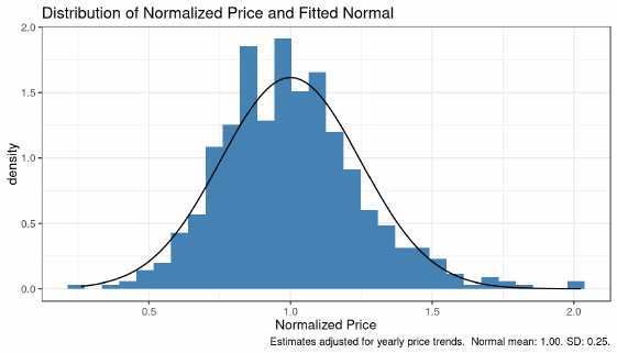
Figure 3: Distribution of resale prices normalized by team-mean in the sample.

Adjusted for yearly trends. From SeatGeek annual average resale prices (76

teams, 576 team-seasons).

Figure 4: Scatterplot of reported willingness to pay with a vaccine and change

in willingness to pay if there is no vaccine.

N Consumers

t = 1 arrivals t = 2 arrivals

Buy ST

Don’t buy ST

Have tickets

Don’t have tickets

(1 − a)N

Don’t resell

Resell

No Purch.

Primary Mkt.

Resale Mkt.

Attend

Don’t attend

t = 1

begins

, p

set

choices

t = 2

begins

Shocks

realized

Purchase

decisions

Game

arrives

Figure 5: Model timeline and outline for consumer arrivals and choices. Deci-

sions are shown in blue.

Parameter Description Notation Estimate Std. Err.

Resale Fee (%) τ 0.22 -

Idiosyncratic Shock Rate ψ 0.08 -

% in First Period a 0.77 -

Preference for Game 1 α

1.00 -

Preference for Game 2 α

1.67 0.032

Preference for Game 3 α

1.01 0.023

Preference for Game 4 α

1.60 0.029

Preference for Game 5 α

0.56 0.015

Preference for Quality 1 γ

0.00 -

Preference for Quality 2 γ

-12.05 0.581

Preference for Quality 3 γ

-17.58 0.55

Preference for Quality 4 γ

-22.65 0.62

Preference for Quality 5 γ

-21.95 0.687

SD of Common Value σ

7.85 0.231

Table 2: Estimated parameters from the ﬁrst stage.

Table 3: Expected state probabilities in September 2021

State Probability

Vaccine 0.59

No Vaccine 0.41

Table 4: Estimated preference change parameters.

Parameter Value Std. Err

NoVax

0.29 0.02

NoVax

52.27 4.50

Vax

0.60 0.02

Vax

43.20 4.58

Table 5: Estimated parameters from the second stage.

Parameter Description Notation Estimate Standard Error

Mean Resale Friction λ

51.43 1.56

Mean Consumer Type λ

16.45 0.11

Mean ST Beneﬁts δ 21.89 1.46

Resale Refunds Flex. Prices No Reall.

Proﬁt (mn) 7.23 7.38 7.50 7.03

(0.09) (0.09) (0.09) (0.08)

Consumer Welfare (mn) 2.64 2.64 2.70 2.47

(0.04) (0.04) (0.04) (0.04)

Total Welfare (mn) 9.97 10.02 10.21 9.49

(0.12) (0.12) (0.12) (0.11)

Resale Fees (mn) 0.10 0.00 0.00 0.00

(0.00) (0.00) (0.00) (0.00)

Season Ticket Buyers (1000) 25.56 26.35 25.72 24.80

Season Ticket Base Price 32.38 30.45 30.90 31.40

Single Game Base Price 39.18 38.59 35.70 40.69

Table 6: Counterfactual results for the baseline model. Standard errors shown

in parentheses.

No Reall. Menu of Refunds Resale

Proﬁt (mn) 6.62 7.17 6.86

(0.08) (0.08) (0.07)

Consumer Welfare (mn) 2.52 2.59 2.38

(0.04) (0.04) (0.09)

Total Welfare (mn) 9.13 9.76 9.25

(0.11) (0.11) (0.12)

Resale Fees (mn) 0.00 0.00 0.02

(0.00) (0.00) (0.00)

Non-Refund. S. Tix (1000) 24.60 12.06 24.60

Vaccine S. Tix (1000) 0.00 5.79 0.00

No Vaccine S. Tix (1000) 0.00 13.10 0.00

Table 7: Counterfactual results for the model with diﬀerent states of the world.

Standard errors shown in parentheses.

Resale τ = 0 λ

= 0 τ = 0 and λ

= 0

Proﬁt (mn) 7.23 7.33 7.28 7.17

(0.09) (0.09) (0.09) (0.09)

Consumer Welfare (mn) 2.64 2.65 2.66 3.13

(0.04) (0.04) (0.04) (0.19)

Total Welfare (mn) 9.97 9.98 10.14 10.30

(0.12) (0.12) (0.13) (0.18)

Resale Fees (mn) 0.10 0.00 0.20 0.00

(0.00) (0.00) (0.01) (0.00)

Season Ticket Buyers (1000) 25.56 25.56 26.19 28.18

Season Ticket Base Price 32.38 32.81 33.50 31.91

Single Game Base Price 39.18 38.68 34.23 27.61

Table 8: Counterfactual results for resale frictions in the baseline model. Stan-

dard errors shown in parentheses.

A Example Details

This section provides illustrations and derivations of the equilibria of

the examples in Section 2. Recall that there is one ticket to be sold over

two periods, that the seller commits to a menu of prices at the start of

the ﬁrst period, and that three demand shocks have known distributions

in the ﬁrst period and known realizations in the second. Consumer i

has value u

= ν

+ V − b

(ω) and consumers incur a friction s when

buying in the resale market.

A.1 Diagrams

Figures 6, 7, and 8 illustrate the main implications of Section 2. The

diagrams, however, do not explicitly illustrate resale’s fees and frictions.

WTP

Time

Alice

enters,

buys

Schedule

conﬂicts

realized

Alice

Bob

enters

Bob

Figure 6: An illustration of the example with only idiosyncratic uncertainty.

Although Alice receives an idiosyncratic shock, Bob does not and is willing to

purchase the ticket at price p.

WTP

Time

Alice

enters,

buys

Schedule

conﬂicts

realized

Star

player

injured

Alice

Bob

enters

Bob

Figure 7: An illustration of the example with idiosyncratic and common value

uncertainty. Alice receives an idiosyncratic shock and an aggregate shock

lowers both her and Bob’s values. Bob is unwilling to pay the primary seller’s

price p, but would purchase directly from Alice for a lower price.

WTP

Time

Purchases

made

State

realized

Alice (ω

, ω

)

E(V

)

Bob (ω

)

Bob (ω

)

F R

(ω

)

F R

(ω

)

Figure 8: An illustration of the example with states of the world. Alice has

the highest value in state ω

and Bob has the highest value in state ω

A.2 Idiosyncratic Uncertainty

Partial Refunds. The optimal price in the second period is p

= 40. In

the ﬁrst period, Alice knows that she will earn zero surplus by waiting to

purchase so she can be charged up to her expected surplus from buying

in the ﬁrst period,

= (1 − ψ) · 50 + ψr. (17)

Any (p

, r) pair with 0 ≤ r ≤ 50 satisfying the expression achieves

the same ﬁnal allocation, proﬁt, and welfare. For simplicity, suppose

that the seller oﬀers r = 5, leaving p

= 41. Alice purchases the ticket.

With probability

, Alice does not receive an idiosyncratic shock and

uses the ticket, generating total welfare of 50 and proﬁt of 41. With

probability

, Alice returns the ticket, yielding a net proﬁt of 41−5 = 36

on the ﬁrst sale and 40 when the ticket is sold again to Bob. The total

proﬁt in this case is 76 and welfare is 40. Expected proﬁt and welfare

are 48.

Resale. The seller sets p

= 40 to ensure that Alice purchases in the

ﬁrst period.

Alice knows that if she receives a shock, she can resell to

Bob for 39. Total welfare is thus .8 · 50 + .2 · 39 = 47.8.

When reselling, Alice sets p

= 39 and receives (1 − .1)39 = 35.1.

She is thus willing to pay

= (1 − ψ) · 50 + ψp

= 40 +

35.1 = 47.02. (18)

The seller can again extract all of Alice’s surplus and sets p

= 47.02,

earning proﬁt of 47.02.

A.3 Idiosyncratic and Common Value Uncer-

tainty

Suppose there is also an aggregate shock: V = 0 with probability

and

V = −20 with probability

Doing so is optimal because the seller wants to sell to Alice in the ﬁrst period: expected

proﬁt exceeds 40 when p

= 40.

Partial Refunds. The seller again oﬀers p

= 40.

In the ﬁrst period,

it can charge Alice

= (1 − ψ)(

· 50 +

· 30) + ψr, (19)

where 0 ≤ r ≤ 30 so that Alice only returns the ticket after an idiosyn-

cratic shock. There are again many optimal pairs of (p

, r). Without

loss of generality, the seller oﬀers r = 5 and charges p

= 37.

Alice contributes 37 to proﬁt and 45 (in expectation) to total welfare

with probability

. The remaining

of the time, the seller earns a net of

32 from Alice and 40 from Bob with probability

and 0 from Bob with

probability

. Proﬁt and total welfare diﬀer from the optimal level

because of the case where Alice returns the ticket and Bob does not

purchase because V = −20 and p

= 40. Expected proﬁt and welfare

both equal 42.

Resale. With resale, the seller sets p

= 40 so that Alice buys the ticket

in the ﬁrst period. If Alice has an idiosyncratic shock she resells to Bob

at price 39 when V = 0, earning 35.1 after fees, or 19 when V = −20,

earning 17.1 after fees. The ticket is always allocated to the consumer

with the highest value, yielding total welfare of

· 45 +

· 34 = 42.8.

The seller’s proﬁt is its price p

, which it sets to extract Alice’s full

surplus,

= (1 − ψ) · (

· 50 +

· 30) + ψ(

· 35.1 +

· 17.1) = 42.12. (20)

A.4 States of the World

The states ω

and ω

each occur with probability

. Alice has value 40

in each state, but Bob has value 50 in state ω

and 10 in state ω

. All

sales must occur in the ﬁrst period, but the state is not realized until

the second period.

Setting p

= 20 is not optimal because, even if the seller extracted all of Alice’s surplus

in the ﬁrst period, it would prefer to earn

· 40 +

· 0 > 20 when Alice has an idiosyncratic

shock.

No Reallocation. Without reallocation, the seller prefers to sell to Alice

at p = 40 than to Bob at p = 30. Proﬁt and welfare are both 40.

Resale. With resale, Bob can resell to Alice in state ω

at price 40,

earning 36. The seller can thus charge Bob up to

p =

· 50 +

36 = 43. (21)

Proﬁt is 43 and total welfare is maximized at 45.

State-Dependent Refund Contracts. The seller can oﬀer a contract

granting a full refund in state ω

at price 40, which Alice is willing

to purchase, and another granting a full refund in state ω

at price 50,

which Bob is willing to purchase. Total welfare is again maximized at

45. Proﬁt is now

40 +

50 = 45.

B Data Construction

I use StubHub listings to infer the distribution of resale transaction

prices. Resale transaction prices are not directly observable from listings

because the StubHub listings only contain tickets currently available

for sale. I start by inferring transactions from changes in listings. For

example, if the number of tickets oﬀered in a listing falls by two from

one day to the next, then I assume two tickets were purchased at the

last observed price.

The procedure leads to false positives because some listings are re-

moved without being sold. I take two steps to correct them. First, I

remove implausibly expensive transactions.

Second, I compare the

number of inferred and actual transactions at the game-section-time

level and assume that the lowest-price inferred transactions are the true

ones. The removed transactions are generally outliers, either occurring

earlier or containing more seats than typical transactions.

These are deﬁned as transactions sold at more than 1.5 times the 75

percentile of price

for similar quality seats.

Figure 9: Sale types and volumes by quality group.

C Additional Descriptive Evidence

Figure 9 shows the average number of tickets sold (across games) for

each sales format and quality zone. As expected, season tickets are

dominant. The “other” cateogry of tickets is also signiﬁcant, but is

not available to the public. It includes student tickets and tickets for

athletics boosters.

Figure 10 shows the distribution of normalized prices for the fo-

cal university and a random sample of 20 universities. The distribu-

tions demonstrate that within-university price variation is signiﬁcant

and widespread. Nearly all universities have a season where prices are

25% above and 25% below the sample mean.

D Estimation Details

D.1 Distribution of V

The estimation procedure for the distribution of V uses the normalized

prices deﬁned in equation (1),

Figure 10: Distribution of average annual resale prices (normalized by school

mean) for a random sample of 20 schools in similar conferences.

NormPrice

= AvgResalePrice

AvgResalePrice

(1 revisited)

The distribution of V is based on residuals from the regression

NormalizedPrice

= β

Season

+ ε

. (22)

The residuals form the distribution in Figure 3, which can be inter-

preted as percent deviations from mean prices. To recover the magni-

tude of the deviations for the university, I multiply the residuals by the

university’s mean price, which is adjusted to reﬂect time trends for the

relevant year.

To recover σ

, the distribution must be adjusted for the eﬀect of

. The adjustment is necessary because changes in V aﬀect utility and

hence resale prices as α

V . Under the assumptions that changes in V

linearly aﬀect resale prices and that deviations in annual resale prices

are solely due to changes in V ,

NormalizedPrice

− 1 = V

(23)

(NormalizedPrice

− 1)









−1

= V

(24)

where the vector w

sums to one and determines the relative impor-

tance of each game. SeatGeek does not describe how their averages

are computed, so I assume that they are an average of all transactions

on their platform and weight the α

parameters by number of resale

transactions. The resulting standard deviation is 7.85.

D.2 Vaccine Demand

Recall from Section 6 that the estimated distribution of values from

structural estimation, parameterized by λ

, reﬂects demand before covid-

19. The survey results suggest that demand with a vaccine is diﬀerent,

as illustrated in Figure 15.

Section 6 explains how the change in values b

(ω

Vax

) is estimated.

In the application with states of the world, I adjust values to reﬂect the

change by deﬁning

= ν

+ b

(ω

Vax

). (25)

I use the distribution of ν

as the distribution of consumer values in

the application. The value changes b

(ω

NoVax

) are independent of ν

Figure 11 demonstrates that the parametric form of b

(ω) ﬁts the

data.

D.3 Second Stage Details

The second stage of estimation includes a grid of values ν

stretching

from $0 to $198 in increments of $0.10. There are 100 values in the grid

for V , the evenly spaced quantiles from 0.5% through 99.5%. The model

iterates until expected and realized resale prices and primary market

purchase probabilities converge, deﬁned as the maximum resale price

diﬀerence being within $0.01 and the mean primary market purchase

probability for each quality is within 1%.

(a)

(b)

Figure 11: Observed and simulated changes in willingness to pay. Top panel

shows change from 2019 WTP to vaccine WTP. Bottom shows vaccine WTP

to no vaccine WTP.

The weight matrix used in the second stage of estimation has mo-

ment variances on the diagonal and zeros elsewhere. Although the in-

verse covariance matrix is asymptotically optimal for GMM, I am unable

to recover the covariances of most estimation moments because they

come from separate data sources. Even for resale prices for diﬀerent

games, an observation only contains information about one game and

so a sample is not informative about the covariance between games. The

resulting weight matrix is consistent but not asymptotically optimal.

I calculate the variance of each moment using the bootstrap. Resale

prices for each game are the simplest case. The data contain records

of resale transactions and their prices. If there are N

observed resale

transactions for game j, I repeatedly sample N

draws from the popu-

lation of transactions and take the variance of the sample average price

as the variance for game j.

Calculating the variance is less straightforward for season ticket and

primary market quantities because the decision to not purchase is un-

observed. In each bootstrap sample, I suppose that there are M total

consumers and and take M Bernoulli draws with success probability

/M, where N

is the observed number of tickets purchased. I censor

each sample to ensure that no more tickets are sold than are available,

then take the variance of the resulting sample means as the moment

variance.

One concern with this strategy is that the variance depends on the

market size M , which is assumed to be 200,000. If there were no cen-

soring, the variance would follow from M Bernoulli draws with success

probability N

/M,

(1 −

) = N

(1 −

). (26)

The only dependence on M is mild because M is large relative to

the quantity purchased. Consequently, the last term is close to one and

the variance is robust to diﬀerent values of M.

Moment variances are presented in Table 9.

I make two adjustments to model output so that it is comparable to

the estimation moments. First, I only use the model’s predicted resale

Table 9: Variance of estimation moments.

Moment Variance

Season Tickets Sold 19899.16

Avg. Resale Price: Game 1 0.30

Avg. Resale Price: Game 2 0.43

Avg. Resale Price: Game 3 0.31

Avg. Resale Price: Game 4 0.53

Avg. Resale Price: Game 5 0.16

PM Tickets Sold: Game 1 1262.01

PM Tickets Sold: Game 2 3286.64

PM Tickets Sold: Game 3 994.04

PM Tickets Sold: Game 4 2394.55

PM Tickets Sold: Game 5 495.96

prices and quantities for the value of V realized in the data. The model

predicts resale prices and quantities for all possible realizations, but only

the one for the realized V is comparable. Second, I weight resale prices

by the observed average quantity of tickets resold in that quantity for

the season. Weighting is necessary because the model predicts resale at

the game-quality level and the mix of qualities resold aﬀects the resale

price.

D.4 Model Fit

Table 10 and Figures 12 and 13 assess the model ﬁt. Observed and

model-implied resale prices are extremely close. The model captures the

patterns in primary market sales across games, but does not ﬁt them

exactly. The looser ﬁt is expected because there are no game-speciﬁc

quantity parameters. Finally, the model-implied number of season tick-

ets purchased is within 13% of the true value.

Table 10: Observed and model-implied quantities of season tickets.

Moment Model-Implied Observed

Season Tickets Sold 25226 22471

Figure 12: Observed and model-implied resale prices for each game.

Figure 13: Observed and model-implied primary market quantities sold.

D.5 Parameter Standard Errors

Standard errors for the ﬁrst stage are calculated using the bootstrap

and the properties of MLE. The errors for the α

and γ

parameters are

calculated using the bootstrap for samples of resale prices. Similarly,

the standard errors for ρ

NoVax

, ρ

NoVax

, ρ

Vax

, and ρ

Vax

are bootstrapped

using repeated sampling of survey responses. The standard error of σ

follows from maximum likelihood.

Standard errors for structural estimation are also calculated using

the bootstrap. I draw a sample of 50 sets of moments from the covari-

ance matrix used to weight moments in estimation and estimate optimal

parameters for each set. The ﬁrst stage parameters are ﬁxed at their

point estimates.

D.6 Counterfactual Standard Errors

Standard errors for counterfactual estimates such as proﬁt are also cal-

culated using the bootstrap. I evaluate each counterfactual 50 times

using 50 sets of input coeﬃcients. The ideal sampling would draw pa-

rameters from their joint distribution, but the full joint distribution is

unknown since not all parameters are estimated jointly.

I account for the correlation between parameters that are jointly

estimated but assume that draws are independent for parameters that

are estimated separately. For example, draws of (λ

, λ

, δ) are correlated

because they are estimated together; the draws are taken from the set

of bootstrapped parameter estimates. The same is true of draws of

the vector (α, γ). However, values of λ

and each α

are assumed to be

independent because they are taken from separate estimation processes.

D.7 Robustness of a

The parameter a is calibrated as the percentage of tickets sold 30 or

more days in advance. To evaluate its eﬀect on the model, I estimate

the second stage using several alternative values. Results are shown in

Table 11. Changing the value of a has a relatively mild eﬀect on frictions

Figure 14: CDF of realized costs of resale for resale buyers in equilibrium.

and valuations, λ

and λ

, but a signiﬁcant eﬀect on the parameter δ

that calibrates the appeal of season tickets. The change in δ is not

surprising. It helps ﬁt the number of consumers who purchase season

tickets. As the number of consumers who consider season tickets varies

with a, it is only natural that δ must change to match the number of

season ticket buyers in the data.

Table 11: Second-stage parameter estimates for diﬀerent values of a.

a λ

0.60 39.73 14.25 60.51

0.70 47.19 15.13 41.78

0.77 51.43 16.45 21.89

0.85 60.84 18.46 -4.34

E Survey

I surveyed 250 Americans under the age of 50 and 250 Americans aged

50 or over, ultimately receiving a total of 457 usable responses. I dis-

tributed the survey through Proliﬁc.co, an online survey distribution

platform. Respondents were paid $9.34 per hour and live in nine states

that each have one dominant college football team: Arkansas, Georgia,

Louisiana, Michigan, Minnesota, Nebraska, Ohio, West Virginia, and

Wisconsin. Respondents from each state were asked to consider one

ticket for that team throughout the survey.

I asked for the amount they are willing and able to pay in four

scenarios: (i) the 2019 season, (ii) a covid-19 vaccine, (iii) no vaccine

but the number of cases falls below the CDC’s near-zero benchmark,

and (iv) no vaccine and the number of cases is above the CDC’s near-

zero benchmark.

The CDC’s benchmark for a near-zero number of new cases is 0.7

new cases per 100,000 people. Respondents were given the benchmark

and a practical illustration, that a 25,000-seat stadium ﬁlled with ran-

domly selected people would contain an average of 2.5 sick people if

each case lasts two weeks. They were also told that the true number of

infected people would be lower, on average, because some people would

know that are ill and decide not to attend.

The survey includes respondents with a wide range of reported WTP.

Figure 15 shows the distribution of reported WTP for three scenarios

without social distancing: a 2019 baseline, a state with a vaccine, and

a state without one. In each state, some consumers report values for

tickets exceeding $50 and $100.

In the absence of a true measure of the probability of each scenario

in the future, I ask respondents how likely they consider each one at

three future dates. The average percent chances are shown in Figure

16. Respondents do not expect a vaccine in January 2021, but think

the chance exceeds 40% in September 2021 and 60% in January 2022.

Figure 17 shows that the distribution of reported WTP is similar

for the near-zero and above near-zero scenarios.

The distributions are

not exactly the same—consumers are more reluctant to attend when

there are more cases—but the diﬀerences are small enough for the two

to be consolidated into a single state without a vaccine. I consolidate

The ﬁgure shows reported WTP without social distancing. The analogous ﬁgure with

social distancing is similar.

Figure 15: Distribution of reported willingness to pay without social distancing

in 2019, with a vaccine, and with no vaccine.

Figure 16: Average reported percent chance of each scenario occurring in each

month.

WTP as a weighted average, taking the relative probability of the states

in September 2021 as the weights.

Figure 17: WTP distributions with near-zero and above near-zero levels of

cases.

Figure 18 shows that the distribution of reported WTP is also similar

with and without social distancing. As before, there are some changes,

but they are not large enough to treat separately. I use reported values

without social distancing because distancing would greatly reduce the

number of tickets the seller can oﬀer.

Surprisingly, demographics were not an important determinant of

the change in WTP across states. I evaluated regression models of the

form

∆WTP

= αAge

+ βRace

+ γState

+ ε

, (27)

where Age

is a set of age dummies (with decade-long bins, e.g. ages

30 − −39), Race

is a set of dummies for race, and State

is a dummy

for the state of the respondent. The response variable is measured both

as an absolute number of dollars and as a percentage of initial WTP.

Lower values denote greater sensitivity to the state without a vaccine.

Results are shown in Table 12.

Table 12: Regression output for equation (27).

Dependent variable:

Value DIﬀerence Value Diﬀerence (%)

(1) (2)

Age 30-39 −12.821 −0.220

(8.713) (0.088)

Age 40-49 −12.419 −0.051

(8.806) (0.089)

Age 50-59 −19.863 −0.169

(8.911) (0.090)

Age 60-69 −7.068 −0.125

(9.574) (0.097)

Age 70-79 −10.209 −0.390

(10.736) (0.109)

Asian 28.256 −0.156

(33.078) (0.335)

African American 43.199 −0.267

(32.337) (0.328)

Other 35.790 −0.495

(36.947) (0.374)

White 50.867 −0.034

(30.960) (0.314)

White, Asian −36.666 −0.078

(60.378) (0.612)

White, African American 74.146 0.447

(48.460) (0.491)

Constant −59.122 −0.213

(32.724) (0.331)

State Fixed Eﬀects Yes Yes

Observations 382 382

0.070 0.114

Adjusted R

0.013 0.060

Residual Std. Error (df = 359) 41.706 0.422

F Statistic (df = 22; 359) 1.233 2.105

∗∗∗

Note: Age coeﬃcients relative to respondents aged 22–29.

Race coeﬃcients relative to respondents who are

American Indians or Alaska Natives.

Although all groups were more sensitive than the reference group of

respondents aged 22–29, those aged 50 and over did not report greater

sensitivity to the state without a vaccine than those aged 30–49. (Re-

spondents 70–79 are not numerous and only show a stronger response

in one model.) Responses vary by race, but no coeﬃcients are signiﬁ-

cant and the groups with large changes have few respondents. Because

the covariance of value diﬀerences with demographics is not a critical

feature of the data, I make value changes independent in the empirical

model.

The full survey is included below.

Page

Event Expectations (General)

Start of Block: Intro

Q1 This study is conducted by Drew Vollmer, a doctoral student researcher, and his advisor, Dr.

Allan Collard-Wexler, a faculty researcher at Duke University.

The purpose of the research is to design sales strategies that cope with uncertainty over the

covid-19 pandemic. You will be asked about how much you would pay for tickets to an outdoor

college football game under several scenarios related to covid-19. The survey should take 5-10

minutes.

We do not ask for your name or any other information that might identify you. Although

collected data may be made public or used for future research purposes, your identity will

always remain confidential.

Your participation in this research study is voluntary. You may withdraw at any time and you

may choose not to answer any question. You will not be compensated for participating.

If you have any questions about this study, please contact Drew Vollmer. For questions about

your rights as a participant contact the Duke Campus Institutional Review Board at

[email protected].

End of Block: Intro

Start of Block: Block 4

Q16 In which state do you currently reside?

▼ Alabama (1) ... I do not reside in the United States (53)

End of Block: Block 4

Start of Block: WTP

Page

In this section of the survey, you will be asked how much you are willing and able to pay for

one ticket to a football game. Your responses should be dollar amounts.

In some questions, you will be given a scenario related to COVID-19. You should respond with

the amount you would pay if that scenario occurs. You should not consider how likely the

scenario is.

Q3 What is the maximum you would be willing and able to pay for one ticket...

Amount (dollars) (1)

one year ago, in Fall 2019? (1)

if there had not been a global COVID-19

outbreak and the virus had not spread to the

US? (2)

if there is a widely available COVID-19

vaccine? (3)

In the next two questions, suppose that there is no COVID-19 vaccine, but that fans are

allowed to attend sporting events.

You will be asked to consider two levels of risk from the virus:

The CDC says that new cases are near zero. The CDC says that new cases are more than

near zero, but risk is low enough to allow fans at sports games.

Page

The CDC standard for new cases to be near zero is 0.7 new cases per 100,000 people or

fewer. This means that filling a 25,000-seat stadium with randomly selected people would imply

an average of 2.5 sick people in the stadium if each case lasts two weeks. The true number of

infected people at any event, however, would be lower because some people would know they

are sick and would not attend.

Suppose that there is no social distancing in the stadium.

What is the maximum you would be willing and able to pay for one ticket if...

Amount (dollars) (1)

the CDC says that the number of new cases is

near zero

? (4)

the CDC says that the number of new cases is

higher than near-zero, but that the risk from

attending mass gatherings is low enough to

allow fans at sports games? (5)

Suppose that there is social distancing in the stadium.

Page

What is the maximum you would be willing and able to pay for one ticket if...

Amount (dollars) (1)

the CDC says that the number of new cases is

near zero

? (4)

the CDC says that the number of new cases is

higher than near-zero, but that the risk from

attending mass gatherings is low enough to

allow fans at sports games? (5)

Suppose that fans can return their tickets if the number of new virus cases is higher than near-

zero. Tickets are sold out, but there is a wait list in case fans who bought tickets return them

because of the virus.

What is the maximum you would be willing to pay for a ticket on the wait list?

Amount (dollars) (1)

No social distancing in the stadium (1)

Social distancing in the stadium (3)

Page

End of Block: WTP

Start of Block: Probabilities

In this section, you will be asked about the likelihood of COVID-19 scenarios. Your answers

should be percent chances. So, if you believe an outcome has a one-in-four chance of

occurring, the percent chance is 25%.

Q34 What is the percent chance of each outcome in January 2021? Chances must sum to

100.

Current total: 0 / 100

_______ There is a widely available COVID-19 vaccine. (1)

_______ There is no COVID-19 vaccine and new cases are near zero, as defined by the CDC.

(2)

_______ There is no COVID-19 vaccine and new cases are higher than near-zero, but the

CDC considers the risk from mass gatherings is low enough to allow fans at sports games. (3)

_______ There is no COVID-19 vaccine, new cases are higher than near-zero, and the CDC

judges that the risk from mass gatherings is high enough that fans cannot attend sports

games. (4)

Q36 What is the percent chance of each outcome in September 2021? Chances must sum to

100.

Current total: 0 / 100

_______ There is a widely available COVID-19 vaccine. (1)

_______ There is no COVID-19 vaccine and new cases are near zero, as defined by the CDC.

(2)

_______ There is no COVID-19 vaccine and new cases are higher than near-zero, but the

CDC considers the risk from mass gatherings is low enough to allow fans at sports games. (3)

_______ There is no COVID-19 vaccine, new cases are higher than near-zero, and the CDC

judges that the risk from mass gatherings is high enough that fans cannot attend sports

games. (4)

Page

Q35 What is the percent chance of each outcome in January 2022? Chances must sum to

100.

Current total: 0 / 100

_______ There is a widely available COVID-19 vaccine. (1)

_______ There is no COVID-19 vaccine and new cases are near zero, as defined by the CDC.

(2)

_______ There is no COVID-19 vaccine and new cases are higher than near-zero, but the

CDC considers the risk from mass gatherings is low enough to allow fans at sports games. (3)

_______ There is no COVID-19 vaccine, new cases are higher than near-zero, and the CDC

judges that the risk from mass gatherings is high enough that fans cannot attend sports

games. (4)

End of Block: Probabilities

Start of Block: Demographics

Q12 What is your year of birth?

________________________________________________________________

Q13 What is your gender?

o Male (1)

o Female (2)

o Prefer not to answer (3)

Q14 What is your ethnicity?

o Hispanic or Latino/Latina (1)

o Not Hispanic or Latino/Latina (2)

Page

Q15 What is your race?

White (1)

Black or African American (2)

American Indian or Alaska Native (3)

Asian (4)

Native Hawaiian or Pacific Islander (5)

Other (6) ________________________________________________

End of Block: Demographics

Figure 18: WTP distributions with near-zero and above near-zero levels of

cases.