HILDA User Manual – Release 10 Michelle Summerfield, Ross

HILDA User Manual – Release 10

Michelle Summerfield, Ross Dunn, Simon Freidin,

Markus Hahn, Peter Ittak, Milica Kecmanovic, Ning Li,

Ninette Macalalad, Nicole Watson, Roger Wilkins, Mark

Wooden

Last modified 07/09/2012

The HILDA Project was initiated, and is funded, by the Australian Government

Department of Families, Housing, Community Services and Indigenous Affairs

HILDA User Manual – Release 10 - ii - Last modified: 7/09/2012

Acknowledgements

Ross Dunn, Alison Goode, Clinton Hayes, Bruce Headey, Rosslyn Starick and Claire

Sun have also contributed to parts of this manual over time.

Simon Freidin prepared the HILDA Data Files in consultation with Mark Wooden,

Nicole Watson, Roger Wilkins and Bruce Headey. The following people provided

database support: Paul Agius, Ross Dunn, Peter Ittak, Ninette Macalalad, Michelle

Summerfield and Diana Warren. The weighting and imputation system was

developed by Nicole Watson, Clinton Hayes, Ning Li, Rosslyn Starick and Claire Sun

in consultation with the HILDA Technical Reference Group (John Henstridge,

Stephen Horn, Frank Yu, Robert Breunig, Peter Boal and Tim Fry).

Citation

Readers wishing to cite this document should use the following:

Summerfield, M., Dunn, R., Freidin, S., Hahn, M., Ittak, P., Kecmanovic, M., Li, N.,

Macalalad, N., Watson, N., Wilkins, R. and Wooden, M. (2011), ‘HILDA User Manual

– Release 10’, Melbourne Institute of Applied Economic and Social Research,

University of Melbourne.

HILDA User Manual – Release 10 - iii - Last modified: 7/09/2012

Updates to This Manual

Date

Update

07/09/12

Amended Financial Year Household income graph connector lines

25/11/11

Updated Manual for Release 10

12/08/11

Updated Section 3.10.1 Numeric Variables and Appendix 1b:source

for W1: D1 Attitudes about work and gender roles

16/05/11

Updated Footnote on table 4.2 to say refer to Selected Standard

Classification pdf for framework (following user query).

03/05/11

Updated response rates for W10 after final report.

06/12/10

Updated Manual for Release 9.

HILDA User Manual – Release 10 iv Last modified: 6/12/11

Contents

1 USING THIS MANUAL............................................................................................................................. 1

2 OVERVIEW OF THE HILDA SURVEY ................................................................................................. 2

2.1 THE HILDA SAMPLE AND FOLLOWING RULES: A SUMMARY................................................................... 2

2.2 QUESTIONNAIRES ...................................................................................................................................... 3

2.2.1 Household Form ............................................................................................................................. 4

2.2.2 Household Questionnaire ............................................................................................................... 4

2.2.3 Person Questionnaires .................................................................................................................... 4

2.2.4 Self-Completion Questionnaire ....................................................................................................... 5

3 THE HILDA DATA .................................................................................................................................... 7

3.1 ORDERING THE DATA................................................................................................................................ 8

3.2 CROSS-NATIONAL EQUIVALENT FILE (CNEF) .......................................................................................... 8

3.3 A REMINDER OF THE SECURITY REQUIREMENTS FOR THE DATA .............................................................. 8

3.4 HOW THE DATA FILES ARE PROVIDED ...................................................................................................... 9

3.5 STRUCTURE OF THE DATA FILES ............................................................................................................. 10

3.6 IDENTIFIERS AND USEFUL VARIABLES .................................................................................................... 10

3.7 PROGRAM LIBRARY ................................................................................................................................ 12

3.7.1 Match Files ................................................................................................................................... 13

3.7.2 Add Partner Variables .................................................................................................................. 13

3.7.3 Create Longitudinal Files ............................................................................................................. 13

3.7.4 User Provided Programs .............................................................................................................. 14

3.8 PANELWHIZ ............................................................................................................................................ 14

3.9 VARIABLE NAME CONVENTIONS ............................................................................................................ 15

3.10 MISSING VALUE CONVENTIONS ......................................................................................................... 20

3.10.1 Numeric Variables ................................................................................................................... 20

3.10.2 Text Variables .......................................................................................................................... 21

3.11 DATA WITH NEGATIVE VALUES ........................................................................................................ 21

3.12 CONFIDENTIALISATION ...................................................................................................................... 22

4 DERIVED VARIABLES .......................................................................................................................... 23

4.1 AGE AND SEX .......................................................................................................................................... 23

4.2 HISTORY ................................................................................................................................................. 24

4.3 GEOGRAPHY............................................................................................................................................ 28

4.4 CURRENT EDUCATION............................................................................................................................. 30

4.5 CURRENT MARITAL STATUS AND DEFACTO RELATIONSHIPS .................................................................. 31

4.6 CHILDREN ............................................................................................................................................... 31

4.7 CHILD CARE ............................................................................................................................................ 32

4.8 OCCUPATION AND INDUSTRY .................................................................................................................. 37

4.9 OTHER EMPLOYMENT ............................................................................................................................. 40

4.10 CALCULATING HOURLY WAGE RATES ............................................................................................... 42

4.11 EMPLOYMENT AND EDUCATION CALENDAR ...................................................................................... 43

4.12 FAMILY RELATIONSHIPS .................................................................................................................... 43

4.13 HEALTH .............................................................................................................................................. 48

4.14 TIME USE ........................................................................................................................................... 50

4.15 PERSONALITY ..................................................................................................................................... 50

4.16 RELIGION ........................................................................................................................................... 51

4.17 INCOME .............................................................................................................................................. 51

4.17.1 Income, Tax and Family Benefits Model .................................................................................. 51

4.17.2 Imputation Method ................................................................................................................... 61

4.17.3 Imputed Income Variables ....................................................................................................... 63

4.18 WEALTH (SPECIAL TOPIC IN WAVES 2, 6 AND 10) .............................................................................. 66

4.18.1 Wealth Model ........................................................................................................................... 66

4.18.2 Imputation Method ................................................................................................................... 69

4.18.3 Imputed Wealth Variables ........................................................................................................ 71

4.19 EXPENDITURE ..................................................................................................................................... 73

4.19.1 Imputation Method ................................................................................................................... 73

4.19.2 Imputed Household Expenditure Variables ............................................................................. 75

HILDA User Manual – Release 10 v Last modified: 6/12/11

4.20

WEIGHTS ............................................................................................................................................ 77

4.20.1 Cross-Sectional Weights .......................................................................................................... 77

4.20.2 Longitudinal Weights ............................................................................................................... 78

4.20.3 Benchmarks .............................................................................................................................. 78

4.20.4 Replicate Weights ..................................................................................................................... 80

4.20.5 Weights Provided on the Data Files ........................................................................................ 80

4.20.6 Advice on Using Weights ......................................................................................................... 83

5 DOCUMENTATION ................................................................................................................................ 87

5.1 DOCUMENTATION CHOICES .................................................................................................................... 87

5.2 MARKED-UP QUESTIONNAIRES ............................................................................................................... 87

5.3 VARIABLE LISTINGS ................................................................................................................................ 88

5.3.1 Subject Listing .............................................................................................................................. 88

5.3.2 Cross-Wave Variable Listing ........................................................................................................ 89

5.3.3 Selected Standard Classifications ................................................................................................. 89

5.4 FREQUENCIES .......................................................................................................................................... 89

5.5 ON-LINE DATA DICTIONARY ................................................................................................................... 90

6 DATA QUALITY ISSUES ....................................................................................................................... 91

6.1 SUMMARY OF DATA QUALITY ISSUES ..................................................................................................... 91

6.2 MISSING INCOME DATA ........................................................................................................................ 100

6.3 MISSING WEALTH DATA ....................................................................................................................... 104

6.4 MISSING EXPENDITURE DATA ............................................................................................................... 108

7 THE HILDA SAMPLE........................................................................................................................... 111

7.1 SAMPLE DESIGN .................................................................................................................................... 111

7.1.1 Overview ..................................................................................................................................... 111

7.1.2 Reference Population .................................................................................................................. 111

7.1.3 Sampling Units ............................................................................................................................ 112

7.1.4 Sample Selection ......................................................................................................................... 113

7.2 FOLLOWING RULES ............................................................................................................................... 113

8 DATA COLLECTION ........................................................................................................................... 114

8.1 PILOT TESTING ...................................................................................................................................... 114

8.2 DEPENDANT DATA ................................................................................................................................ 114

8.3 QUESTIONNAIRE LENGTH...................................................................................................................... 115

8.4 INTERVIEWERS ...................................................................................................................................... 115

8.5 FIELDWORK PROCESS............................................................................................................................ 116

8.5.1 Data Collection Mode ................................................................................................................. 116

8.5.2 Timeline ...................................................................................................................................... 117

8.5.3 Survey Notification Material....................................................................................................... 118

8.5.4 Respondent Incentives ................................................................................................................. 119

8.5.5 Call Routine, Follow-Up and Refusal Aversion .......................................................................... 119

8.5.6 Foreign Language Interviews ..................................................................................................... 120

8.5.7 Interviewer Monitoring ............................................................................................................... 120

8.6 RESPONSE RATES .................................................................................................................................. 120

8.7 ATTRITION BIAS .................................................................................................................................... 129

9 HILDA USER TRAINING ..................................................................................................................... 132

10 GETTING MORE INFORMATION .................................................................................................... 133

11 REFERENCES ........................................................................................................................................ 134

APPENDIX 1A: SUMMARY OF HILDA SURVEY CONTENT, WAVES 1 – 10 .................................... 138

APPENDIX 1B: SURVEY INSTRUMENT DEVELOPMENT AND SOURCES ...................................... 148

APPENDIX 1C: LIST OF ACRONYMS USED ............................................................................................ 164

APPENDIX 2: IMPUTATION METHODS USED IN THE HILDA SURVEY ......................................... 165

NEAREST NEIGHBOUR REGRESSION METHOD ................................................................................................ 165

LITTLE AND SU METHOD ................................................................................................................................ 165

HILDA User Manual – Release 10 vi Last modified: 6/12/11

OPULATION CARRYOVER METHOD ............................................................................................................... 166

HOTDECK METHOD ........................................................................................................................................ 167

HILDA User Manual – Release 10 vii Last modified: 6/12/11

List of Figures

Figure 2.1: The evolution of the HILDA Survey sample across the first three waves ................... 3

Figure 4.1: Family where a new defacto relationship is formed

.................................................... 45

Figure 4.2: Family where a new child is born

................................................................................... 45

Figure 4.3: Construction of family type description

........................................................................ 46

Figure 4.4: Construction of household type description

................................................................ 46

Figure 4.5: Income units in a family with child under 15, dependent student and non-dependent

children

............................................................................................................................... 47

Figure 4.6: Financial year income model (household-level)

........................................................... 56

Figure 4.7: Financial year income model (enumerated person-level)

........................................... 57

Figure 4.8: Financial year income model (responding-level)

......................................................... 58

Figure 4.9: Wealth model (household-level)

..................................................................................... 68

Figure 5.1: Example of the marked-up questionnaires

................................................................... 88

Figure 5.2:: Example of the subject listing

....................................................................................... 88

Figure 5.3: Example of the cross-wave variable listing (wave 7, 8, 9 and 10 truncated)

............. 89

Figure 5.4: Example of the frequencies

............................................................................................ 89

HILDA User Manual – Release 10 viii Last modified: 6/12/11

List of Tables

Table 2.1: Actual and proposed structure of the HILDA questionnaire modules .......................... 2

Table 2.2: Sections of the Person Questionnaires

............................................................................ 5

Table 2.3: Sections of the Self-Completion Questionnaire

............................................................... 6

Table 3.1: Total number of HILDA data users, Release 1 to 9

.......................................................... 7

Table 3.2: HILDA data users by type, Release 1 to 9

......................................................................... 7

Table 3.3: List of useful variables

..................................................................................................... 12

Table 3.4: Broad subject area naming conventions, characters 2 and 3 (sorted by code)

......... 16

Table 3.5: Different codes for household response status

............................................................ 17

Table 3.6: Different codes for person response status

................................................................... 18

Table 3.7: Different codes for SCQ field response status

.............................................................. 19

Table 3.8: Different codes for household membership

................................................................... 19

Table 3.9: Different codes for new location of mover

..................................................................... 20

Table 3.10: Missing value conventions for numeric variables

....................................................... 20

Table 3.11: Missing value conventions for text variables

............................................................... 21

Table 4.1: History variables

............................................................................................................... 24

Table 4.2: Derived geographic variables

.......................................................................................... 29

Table 4.3: Derived current education variables

............................................................................... 30

Table 4.4: Derived current marital status and defacto relationship variables

.............................. 31

Table 4.5: Derived children variables

................................................................................................ 32

Table 4.6: Child care variables

.......................................................................................................... 34

Table 4.7: Derived occupation and industry variables

.................................................................... 39

Table 4.8: Other derived employment variables

.............................................................................. 41

Table 4.9: Derived employment and education calendar variables

............................................... 43

Table 4.10: Derived family variables

................................................................................................. 47

Table 4.11: Derived health variables

................................................................................................. 49

Table 4.12: Derived time use variables

............................................................................................. 50

Table 4.13: Derived personality variables

........................................................................................ 51

Table 4.14: Australian resident income tax rates, waves 1 to 10

................................................... 55

Table 4.15: Other derived income variables ..................................................................................... 60

Table 4.16: Percentage of missing cases imputed by imputation method (income), waves 1 to 10

............................................................................................................................................. 62

Table 4.17: Imputed income variables

.............................................................................................. 63

Table 4.18: Other derived wealth variables at household-level

..................................................... 69

Table 4.19: Percentage of missing cases imputed by imputation method (wealth), waves 2, 6, and

......................................................................................................................................... 71

Table 4.20: Percentage of missing cases imputed by imputation method (home value), waves 1

to 10

..................................................................................................................................... 71

Table 4.21: Imputed wealth variables

................................................................................................ 72

Table 4.22: Percentage of missing cases imputed by imputation method (expenditure), waves 1

to 10

..................................................................................................................................... 75

Table 4.23: Imputed household expenditure variables

................................................................... 76

Table 4.24: Benchmarks used in weighting

..................................................................................... 80

Table 4.25: Weights

............................................................................................................................. 81

Table 4.26: Sample design variables

................................................................................................ 85

Table 6.1: Summary of the data quality issues in the HILDA data

................................................. 91

Table 6.2: Proportion of cases with missing income data, waves 1 to 10 (per cent)

................. 101

HILDA User Manual – Release 10 ix Last modified: 6/12/11

Table 6.3: Mean financial year income ($) (including imputed values) and percent of mean

income imputed, waves 1 to 10 (weighted)

................................................................... 104

Table 6.4: Cases with missing wealth data including and excluding wealth band responses,

waves 2, 6 and 10 (per cent)

........................................................................................... 105

Table 6.5: Households with missing home value data, waves 1 to 10 (per cent)

....................... 107

Table 6.6: Mean wealth value ($) (including imputed values) and percentage of mean value

imputed, waves 2, 6 and 10 (weighted)

......................................................................... 107

Table 6.7: Mean home value ($’000) (including imputed values) and percentage of mean value

imputed, waves 1 to 10 (weighted)

................................................................................ 108

Table 6.8: Households with missing expenditure data, wave 1 – 10 (per cent)

.......................... 108

Table 6.9: Mean expenditure and percentage of mean expenditure imputed, wave 1 – 10

(weighted)

......................................................................................................................... 110

Table 8.1: Average time (minutes) taken to complete questionnaires, waves 1 to 8

................. 115

Table 8.2: Number of interviewers and percentage of new interviewers each wave

................. 116

Table 8.3: Percentage of respondents interviewed by telephone

................................................ 116

Table 8.4: Fieldwork dates and percentage of interviews post December

................................. 117

Table 8.5: Distribution of individual interviews conducted by month, waves 1 to 10

............... 118

Table 8.6: Distribution of individual interviews conducted around the anniversary of the prior

wave’s interview, waves 2 to 10

..................................................................................... 118

Table 8.7: Wave 1 household outcomes

......................................................................................... 121

Table 8.8: Wave 1 person outcomes

............................................................................................... 121

Table 8.9: Wave 2 household outcomes

......................................................................................... 122

Table 8.10: Wave 3 household outcomes

....................................................................................... 122

Table 8.11: Wave 4 household outcomes

....................................................................................... 123

Table 8.12: Wave 5 household outcomes

....................................................................................... 123

Table 8.13: Wave 6 household outcomes

....................................................................................... 124

Table 8.14: Wave 7 household outcomes

....................................................................................... 124

Table 8.15: Wave 8 household outcomes

....................................................................................... 125

Table 8.16: Wave 9 household outcomes

....................................................................................... 125

Table 8.17: Wave 10 household outcomes

..................................................................................... 126

Table 8.18: Wave 2 to 10 person outcomes against wave 1 person outcomes

.......................... 127

Table 8.19: Individual response rates for the HILDA Survey, waves 2 to 10 compared

............ 128

Table 8.20: Self Completion Questionnaire response rate, wave 1 to 10

.................................... 129

Table 8.21: Percentage of wave 1 respondents re-interviewed by selected sample characteristics

........................................................................................................................................... 131

HILDA User Manual – Release 10 1 Last modified: 6/12/11

1 USING THIS MANUAL

The HILDA Survey is a household-based longitudinal survey named the Household,

Income and Labour Dynamics in Australia Survey. This manual has been designed

for the users of the HILDA data.

The manual aims to cover the things that you need to know to use the HILDA data –

such as missing data conventions, an introduction to the derived variables, how to

put the data files together, imputation, weights and how to find your way around the

documentation.

The best way to use this manual is as a reference tool. It is unlikely that you will sit

down and read it cover to cover and take away everything you need to know about

the data. More realistically, you will start to work with the data and will need some

information about certain aspects of the data or the survey – and hopefully you will

be able to find it within this manual fairly easily.

We welcome any feedback you have on this manual. It will be updated as

successive waves are made available to researchers and we are happy to hear how

it could be improved. If there is something that you expected to find in the manual

and didn’t, or if you had difficulty finding or understanding any section, please let us

know (email hilda-inquiries@unimelb.edu.au).

HILDA User Manual – Release 10 2 Last modified: 6/12/11

2 OVERVIEW OF THE HILDA SURVEY

The HILDA Survey is a broad social and economic longitudinal survey, with

particular attention paid to family and household formation, income and work. As the

HILDA Survey has a longitudinal design, most questions are repeated each year.

Nevertheless, within each survey wave, scope exists for asking questions on topics

that will not be covered every year. The major modules included in the HILDA

Survey are listed in Table 2.1.

Table 2.1: Actual and proposed structure of the HILDA questionnaire modules

Wave

2 3 4 5 6 7 8 9 10 11

Major modules

Wealth X X X

Fertility X X X

Health X

Education / Human capital X

Minor modules

Retirement X X X

Intentions and plans X X X

Non co-residential partners X X X

Non—co-residential parents,

siblings and adult children

X X

Health insurance X X

Youth X

Literacy and numeracy X X

Diet X X

1. The content for waves 11 and 12 is under discussion.

2.1 The HILDA Sample and Following Rules: A Summary

The HILDA Survey began with a large national probability sample of Australian

households occupying private dwellings. All members of the households providing at

least one interview in wave 1 form the basis of the panel to be pursued in each

subsequent wave. The sample has been gradually extended to include any new

household members resulting from changes in the composition of the original

households. From wave 9, new household members that arrived in Australia for the

first time after 2001 were also added to the sample.

Continuing Sample Members (CSMs) are defined to include all members of wave 1

households. Any children subsequently born to or adopted by CSMs are also

classified as CSMs. Further, all new entrants to a household who have a child with a

CSM are converted to CSM status. CSMs remain in the sample indefinitely. All other

HILDA User Manual – Release 10 3 Last modified: 6/12/11

people who share a household with a CSM in wave 2 or later are considered

Temporary Sample Members (TSMs). TSMs are followed for as long as they share a

household with a CSM. The variable hhsm on the master file identifies TSMs while

the CSMs are split into two groups: OSMs (original sample members from wave 1)

and OPMs (other permanent sample members, i.e. ‘new’ CSMs).

Figure 2.1 shows an example of how the sample evolved across the first three

waves. In wave 1, the sample consisted of 19,914 people. A further 442 births and

54 parents of newborns who were not originally CSMs have been added to the

sample in waves 2 and 3. A total of 177 deaths have been identified across the two

follow-up waves and 256 people have moved overseas, though 24 returned after

being away for one wave. Of the TSMs joining the sample in wave 2, a third had

moved out by wave 3.

Figure 2.1: The evolution of the HILDA Survey sample across the first three waves

2.2 Questionnaires

In wave 1, the HILDA survey comprised four different instruments. These were:

HILDA User Manual – Release 10 4 Last modified: 6/12/11

• the Household Form (HF);

• the Household Questionnaire (HQ);

• the Person Questionnaire (PQ); and

• the Self-Completion Questionnaire (SCQ).

In subsequent waves, the PQ was replaced with two instruments:

• the Continuing Person Questionnaire (CPQ), for people who have been

interviewed in a previous wave, and

• the New Person Questionnaire (NPQ), for people who have never been

interviewed before (which collects family background and personal history

information along with the regular content).

Appendix 1a provides a guide to topics covered in the HILDA Survey across the

waves. Appendix 1b provides a list of sources used in constructing survey questions.

The questionnaires can be downloaded from the HILDA website:

http://www.melbourneinstitute.com/hilda/questionnaires/default.html or you can view

the questionnaires provided with the data files which have been marked up with the

associated variable names (see the documentation section later in this manual).

2.2.1 Household Form

The HF is designed to record basic information about the composition of the

household immediately after making contact. The HF is the ‘master document’ used

by interviewers to decide who to interview, how to treat joiners and leavers of the

household, and to record call information and non-interview reasons. The date the

HF is completed is provided in _hhcomps. The number of interviews completed in

the household is given in _hhivws.

2.2.2 Household Questionnaire

The HQ collects information about the household rather than about individual

household members per se, and is only administered to one member of the

household. In practice, however, interviewers are encouraged to be flexible. If more

than one household member wishes to be present at the interview this is perfectly

acceptable. Further, interviewers are given the flexibility to deliver part of this

interview to one household member and part to another. Indeed, this was often

required, with questions on child care needing to be asked of the primary care giver.

The date the HQ is completed is provided in _hhhqivw.

The HQ mainly covers child care arrangements, housing, household spending (until

wave 5) and, in waves 2 and 6, household wealth.

2.2.3 Person Questionnaires

The PQs are administered to every member of the household aged 15 years and

over. The CPQ is for people who have ever been interviewed before and the NPQ is

for those who have never been interviewed before. Parental consent is sought

before interviewing persons aged under 18 years who are still living with their

parents. _hhpq states which type of interview was applicable and _hgwsli indicates

how many weeks have elapsed since the respondent’s last interview (if they are

completing a CPQ). The date the PQ is completed is provided in _hhidate.

HILDA User Manual – Release 10 5 Last modified: 6/12/11

The sections of the person questionnaires are shown in Table 2.2 together with the

letter used to identify the section. These will help you locate questions on the

questionnaires (for example, if you wanted to find questions on education, look in

section C of the wave 1 Person Questionnaire and section A of the Continuing

Person Questionnaire and New Person Questionnaire from wave 2 onwards).

The PQ in wave 1 is distinctive from that used in the later waves as it collected

biographical data that only needs to be asked once. These questions are spread

throughout the survey and include questions about country of birth and language,

family background, educational attainment, employment history, and marital history.

In addition, at later waves further biographical information about visa category for

immigrants (wave 4) and parents’ education (wave 5) was collected.

The NPQ differs from the CPQ in the inclusion of these additional biographical

history questions.

Table 2.2: Sections of the Person Questionnaires

Topics

Section

Wave 2 onwards Wave 1

Country of birth AA (NPQ only, except in wave 4

) A

Family background BB (NPQ only) B

Education A C

Employment status B D

Current employment C E

Persons not in paid employment D D, F

Annual activity calendar E FG

Income F G

Family formation G H

Partnering/relationships H J

Health, life satisfaction, moving K K

Tracking information T T

Interviewer observations Z Z

Special Topics

Wealth (wave 2, 6 and 10) J

Retirement (wave 3 ,7 and 10) L

Private health insurance (wave 4 only) J

Youth issues (wave 4 only) L

Fertility and partnering (wave 5 and 8) G, H

Intentions and Plans (wave 5 and 8) L

1. Immigration Status asked in wave 4 in section AA

2.2.4 Self-Completion Questionnaire

Finally, all persons completing a person questionnaire are asked to complete a Self-

Completion Questionnaire which the interviewer collects at a later date, or failing

that, is returned by mail. This questionnaire comprises mainly attitudinal questions,

many of which cover topics which respondents may feel slightly uncomfortable

answering in a face-to-face interview. The date that the SCQ is completed is not

HILDA User Manual – Release 10 6 Last modified: 6/12/11

collected for waves 1 to 8 (but is included from wave 9). The variable _hhmpid

indicates whether an SCQ has been matched to the PQ.

Table 2.3 shows the sections of the SCQ together with the letter used to identify the

section.

Table 2.3: Sections of the Self-Completion Questionnaire

Topics Wave 1 W5 and 8 Other waves

General health and well-being (SF-36) A A A

Lifestyle and living situation B B B

Personal and household finances C C C

Attitudes and values D D -

Job and workplace issues E E D

Parenting F F E

Sex and age - G F

HILDA User Manual – Release 10 7 Last modified: 6/12/11

3 THE HILDA DATA

The HILDA Survey has already developed a sizeable community of users. Table 3.1

and Table 3.2 show the total number of individuals who have been approved access

to at least one of the data releases and the composition of our user community.

There are also 82 users of the HILDA-Cross-National Equivalent File (HILDA-CNEF).

Table 3.1: Total number of HILDA data users, Release 1 to 9

Release Total data orders Orders by new users Cumulative no. of users

Release 1 204 204 204

Release 2 265 169 373

Release 3 279 157 530

Release 4 329 176 706

Release 5 387 196 902

Release 6 401 176 1078

Release 7 455 199 1277

Release 8 430 124 1401

Release 9 486 131 1532

Table 3.2: HILDA data users by type, Release 1 to 9

Release

Type of user 1 2 3 4 5 6 7 8 9

Academic – Australia 84 112 126 142 169 178 205 199 238

Academic –

Overseas

5 15 18 19 24 25 37 24 52

Students – Honours

year

3 13 16 15 13 7 13 17 13

Students –

Postgraduate

9 16 18 31 42 41 41 44 55

Government –

Australian

87 87 82 103 120 134 137 119 104

Government –

State/Local

8 14 8 11 8 5 10 6 8

Other 8 8 11 8 11 11 12 21 18

Total 204 265 279 329 387 401 455 430 488

HILDA User Manual – Release 10 8 Last modified: 6/12/11

3.1 Ordering the Data

Access to the data can be gained by an Organisational Licence or an Individual

Licence. You MUST be a registered user to use the data. Organisations that are

likely to have more than four individuals who wish to use the HILDA data should

consider signing up to an Organisational Licence as this would provide quicker

access to the data (and at a lower cost) once the Organisational Licence is signed.

Details of how to order the data are provided on the HILDA website:

http://www.melbourneinstitute.com/hilda/data/default.html

3.2 Cross-National Equivalent File (CNEF)

The Cross National Equivalent File originated from a Cornell University project to

create an equivalent set of income measures for the German SOEP and the

American PSID. It has since expanded to include data from many other countries

which are undertaking longitudinal household panels (Australia, Canada, Germany,

Great Britain, Korea, Switzerland and the United States), and the range of data has

expanded to include employment, health and psychological measures. The HILDA-

CNEF files are included on the HILDA DVD, but the password must be obtained from

Cornell.

The current CNEF-HILDA codebooks and details of how to order the CNEF data can

be found at

3.3 A Reminder of the Security Requirements for the Data

http://www.melbourneinstitute.com/hilda/cnef.html.

The Deed of Licence and the Deed of Confidentiality stipulates numerous security

requirements for the data, some of which are outlined below:

• You CANNOT provide the data to any unauthorised individual (to be

authorised, you must have an Individual Deed of Licence countersigned by

the FaHCSIA delegate or have a Deed of Confidentiality countersigned by

your organisation’s approved Data Manager).

• You MUST include the following paragraph in any work written that use the

HILDA data:

This paper uses unit record data from the Household, Income and

Labour Dynamics in Australia (HILDA) Survey. The HILDA Project was

initiated and is funded by the Australian Government Department of

Families, Housing, Community Services and Indigenous Affairs

(FaHCSIA) and is managed by the Melbourne Institute of Applied

Economic and Social Research (Melbourne Institute). The findings and

views reported in this paper, however, are those of the author and

should not be attributed to either FaHCSIA or the Melbourne Institute.

• If you plan to change employers and you have an Individual Deed of

Licence, you MUST contact FaHCSIA before doing so to discuss suitable

arrangements for the data. Under certain conditions you may be able to

take the data with you. Otherwise, you will need to delete any data files

HILDA User Manual – Release 10 9 Last modified: 6/12/11

and destroy the CD/DVD and notify FaHCSIA

(longitudinalsurveys@fahcsia.gov.au) and the Melbourne Institute (hilda-

inquiries@unimelb.edu.au) that you have done so.

• If you plan to change employers and your organisation has an

Organisational Deed of Licence, you MUST contact your organisation’s

Data Manager to resolve your user obligations to the security of the

dataset.

• If you change your research project you MUST first seek permission for

the new project from FaHCSIA.

• The HILDA CD/DVD MUST be kept secure in a locked filing cabinet or

other secure container when not in use.

• The keys or combinations for the filing cabinet or other secure container

must be kept secure and not given to any unauthorised user.

• The HILDA data (and any derivatives of the HILDA data) must be stored

on a password protected computer or network and must not be given to

any unauthorised user.

• Your password MUST be at least 7 characters long, include a mixture of

upper and lowercase characters, contain numbers and some non-

alphanumeric characters such as # ; * or !.

• Any printed unit record output MUST be stored in a locked filing cabinet or

other secure container when not in use. Any printed unit record output

MUST be shredded if no longer required.

• There MUST be a means of limiting access to the work area where the

data is kept and tamper evident barriers to access (i.e., if there were a

break-in, it would be obvious from broken glass, damaged lock, etc).

3.4 How the Data Files are Provided

All data are provided in SAS, SPSS

and STATA (Version 10 and 11)

The DVD also includes extensive documentation of the data, including coding

frameworks, marked-up questionnaires and variable frequencies. The files and the

documentation are discussed in detail in later sections. Changes to the data files

between Releases can be found at:

formats.

http://www.melbourneinstitute.com/hilda/doc/previous_releases.html.

The data files can be transferred to other statistical packages using StatTransfer or

any other data conversion package of your choice.

SPSS portable files can be obtained by special request to

You may need to restrict the

number of variables to be included in your transferred datasets due to the limitations

on the number of variables imposed by some statistical packages.

hilda-inquiries@unimelb.edu.au.

You will need to use STATA SE as there are more than 2047 variables in the datasets. Suitable

memory and maxvar values are provided in “Readme 100.pdf” on the DVD.

A trial copy of StatTransfer Version 10 can be downloaded from www.stattransfer.com or purchased

online at

www.stattransfer.com/html/store.html.

HILDA User Manual – Release 10 10 Last modified: 6/12/11

3.5 Structure of the Data Files

For each wave, there are four files:

• Household File – containing information from the HF and HQ.

• Enumerated Person File – listing all persons in all responding households

and contains limited information from the HF (includes respondents, non-

respondents and children).

• Responding Person File – containing all persons who provided an

interview and contains CPQ/NPQ and SCQ information.

• Combined file – this is a combined file of the three files above. The

household information and responding person information is matched to

each enumerated person.

In addition, a master file and a longitudinal weights file are provided. The master file

contains all persons enumerated at any wave, their interview status in each wave

and limited information about the individual. You can convert the master file to a long

format if you use the rest of the data in long format. The longitudinal weights file

contains weights for all sequential balanced panel combinations and all balanced

pairs of waves.

3.6 Identifiers and Useful Variables

Household and person level files within a wave can be merged by using _hhrhid (i.e.

ahhrhid for wave 1, bhhrhid for wave 2, etc).

Information from enumerated or responding person files can be linked across waves

by using either:

Note that where we use the

underscore ‘_’ in the variable name, you will need to replace it with the appropriate

letter for the wave, ‘a’ for wave 1, ‘b’ for wave 2, etc. Enumerated and responding

person files within a wave can be merged by using the cross-wave identifier xwaveid

or the wave specific person identifier _hhrpid. In wave 1, the first six characters of

_hhrpid is the household identifier and the last two characters of the person identifier

is the person number within the household. In wave 2 onwards, the first five

characters are the household identifier and the next two are the person number.

• the cross-wave identifier xwaveid; or

The variable _hgenum indicates whether the person belonged to a responding household each

wave and this may be useful when selecting those who have been tracked over the entire study

irrespective of whether they were interviewed (enumerated at all waves).

The variable _hgint indicates whether the person completed an interview and this is one way to select a

balanced responding panel (_hgint

=1 at all waves), or to reduce the Combined files into “interviewed adult

only” files (this removes the person level records for children or “non-responding adults from responding

households” which are included to describe the whole Australian population when calculating measures

such as the poverty rate or gini coefficient)..

Users of the In-confidence Release files can alternatively use _hhid to match the household and

person files, and _hhpid to match the person files. In wave 1, the household identifier is six digits long,

corresponding to area (three digits), dwelling number (two digits) and household number (one digit).

The person identifier in wave 1 is then eight digits long – the first six are the household identifier,

followed by two digits for the person number. In subsequent waves, the household identifier is five

digits long, and the person identifier is seven digits long.

HILDA User Manual – Release 10 11 Last modified: 6/12/11

• the master file which shows the identifiers for each person each wave.

Note that while xwaveid is the unique identifier to match each person across all

waves, _hhrhid and _hhrpid are specific identifiers to match each person within a

wave. As _hhrhid and _hhrpid are randomly assigned each wave, the same person

will have a different _hhrhid and _hhrpid from wave to wave. Persons in the same

household in each wave will share the same _hhrhid and the same first 5 digits in

_hhrpid (or the same first 6 digits in ahhrpid in the case of wave 1).

Partners within the household are identified by their cross-wave identifier (_hhpxid)

or by their two digit person number for the household (_hhprtid). These variables are

provided on both the enumerated and responding person files and are derived using

the HF relationship grid. Partners are either married or de-facto and include same

sex couples. _hhprtid is the person number for the household (for example, if person

02’s partner is person 05, the partner identifier for person 02 will contain ‘05’ and for

person 05 it will contain ‘02’). You will need to concatenate the household identifier

with the partner identifier before you can match on partner characteristics to the

person file. Using the partner’s cross-wave identifier (_hhpxid) will be much easier.

Parents within the household are similarly identified in _hhfxid and _hhmxid (father’s

and mother’s crosswave identifiers) or _hhfid (father’s person number) and _hhmid

(mother’s person number). A parent may be natural, adopted, step or foster (a

parent’s de facto partner also counts as a parent).

Listed below in Table 3.3 are some useful socio-demographic variables. These are

provided to help new users get started with using the HILDA data.

HILDA User Manual – Release 10 12 Last modified: 6/12/11

Table 3.3: List of useful variables

Variable Description Variable Description

xwaveid Cross wave person identifier _hhfty Family type

_hhrhid Random household identifier _hhiu Income unit

_hhrpid Random person identifier _hhpxid Partner’s cross-wave identifier

hhsm Sample member type _hhfxid Father’s cross-wave identifier

_hhresp Household response status _hhmxid Mother’s cross-wave identifier

_fstatus Person response status (master file) _hhstate State

_hhpers Number of persons in household _hhsos Section of state

_hhtype Household type _hhmsr Major statistical region

_hhyng Age of youngest person in HH _ancob Country of birth

_hhold Age of oldest person in HH _hgage Age

_hhrih Relationship in household _hgsex Sex

_hhfam Family number _mrcurr Marital status

_esbrd,

_esdtl

Employment status (broad, detail) _losat Life satisfaction

_jbhruc

Combined per week usually worked

in all jobs

_edhigh Highest education level achieved

_jbmo62 Occupation code 2-digit ANZSCO _edfts Full-time student

_wscei

Imputed current weekly gross

wages and salary – all jobs

_edagels Age left school

_wsfei

Imputed financial year gross wages

and salary

_edhists

Highest year of school completed/currently

attending

_hifdip,

_hifdin

Household disposable income

(positive and negative)

_edtypes Type of school attended/attending

_hhda10

SEIFA decile of socio-economic

disadvantage

_helth

Long term health

condition/disability/impairment from PQ

3.7 Program Library

Several programs have been provided on the HILDA website in SAS, SPSS and

Stata to help you get started with the HILDA data. These files are found on

http://www.melbourneinstitute.com/hilda/doc/programlibrary.html

HILDA User Manual – Release 10 13 Last modified: 6/12/11

3.7.1 Match Files

The programs showing how to match files are:

• Program 1 – SAS program to match wave 1 household and responding

person files

• Program 2 – SPSS program to match wave 1 household and responding

person files

• Program 3 – Stata program to match wave 1 household, enumerated and

responding person files

3.7.2 Add Partner Variables

Some users may want to include variables for a respondent’s partner in their

analyses. The programs showing how to utilise the partner’s cross-wave identifier

_hhpxid to add partner variables onto the responding person file are:

• Program 4 – SAS program to add partner variables

• Program 5 – SPSS program to add partner variables

• Program 6 – Stata program to add partner variables

3.7.3 Create Longitudinal Files

There are a number of ways users might want to create a balanced longitudinal file:

• Wide file of responding persons – this is where we keep only people

responding in all waves and put the variables for each wave next to each

other (that is, there is one row of data for each person).

• Wide file of enumerated persons – this is where we keep only those

people who were in responding households in all waves and the variables

for each wave are put next to each other.

• Long file of responding persons – this is where we keep only people

responding in all waves and the information for each wave is stacked

together (that is, there is a separate row of data for each wave of

information for each person).

• Long file of enumerated persons – this is where we keep only those

people who were in responding households in all waves and the

information for each wave is stacked together.

Most users will probably want to restrict the files to only include respondents or

people from responding households. A few users may also want to add people who

have died or moved out of scope (depending on the research question they are

answering).

The programs showing how to create balanced long files of responding persons are:

• Program 7 – SAS program to create long longitudinal files

• Program 8 – SPSS program to create long longitudinal files

The wide files are created by matching the responding or enumerated files for each

wave together using xwaveid. An alternative way to strip off the first letter of the

variable names in SAS is provided in

HILDA User Manual – Release 10 14 Last modified: 6/12/11

• Program 9 – SAS macro to strip the first letter from the variable name

Some users may want to create an unbalanced panel – where you take all

respondents or enumerated persons available at each wave (not just those that

consistently respond or are consistently in responding households). An example

Stata program to create a balanced or unbalanced panel is provided in

• Program 10 – Stata program to create long longitudinal files

Example programs to create wide files are provided in:

• Program 11 – SAS program to create wide longitudinal files

• Program 12 – SPSS program to create wide longitudinal files

• Program 13 – Stata program to create wide longitudinal files

The longitudinal weights on the enumerated person file and the responding person

file are for the full balanced panel of respondents and enumerated persons from

wave 1 (i.e., across the first two, three, … ten waves). If you are constructing a

balanced panel with different specifications, you should find a suitable weight in the

longitudinal weights file. Out of scopes (deaths and moves overseas) are treated as

acceptable outcomes, so these people have weights applied as well.

3.7.4 User Provided Programs

Users of the HILDA data can also contribute code to this library if they believe it may

be beneficial to other users. Please send your code to hilda-

inquiries@unimelb.edu.au.

3.8 PanelWhiz

PanelWhiz is a collection of Stata/SE Add-On scripts to make using panel datasets

easier. PanelWhiz simplifies finding, retrieving and managing variables from multiple

waves (without the need to refer to external documentation or type long lists of

complicated variable names), selecting appropriate weights, matching partner

information and a variety of other common tasks that occur in panel research. By

allowing you to save variable ‘sets’ it also simplifies replacing your working files at

subsequent releases of HILDA data. The package creates a long longitudinal file.

The interface only runs in Stata/SE, but you can export the created datasets into

SPSS, SAS, LIMDEP, GAUSS, and Excel.

For HILDA, PanelWhiz is only available for the General Release Stata files. It uses

the Combined *c.dta file from each wave of the release, plus these files from the

Stata zip: Master_h100c.dta, Longitudinal_weights_h100c.dta; and _version. The

General Release Stata Combined files have PanelWhiz metadata pre-loaded.

PanelWhiz is charityware, requiring the user to make a direct donation to UNICEF.

Details of how to order PanelWhiz can be found at www.panelwhiz.eu.

This program requires at least 1.3gb memory to run. If your computer does not have this much

memory then you will need to restrict the datasets to only the subset of variables you need.

HILDA User Manual – Release 10 15 Last modified: 6/12/11

3.9 Variable Name Conventions

Variable names have been limited to eight characters (so that the files can be read in

older versions of SPSS and SAS). The variable name is divided into three parts and

attempts to provide information on the content of the variables:

• First character – wave identifier, with ‘a’ being used for wave 1, ‘b’ for

wave 2, ‘c’ for wave 3, etc.

• Second and third character – general subject area (see Table 3.4) for the

conventions).

• Fourth to eighth character – specific subject of data item.

Excluding the first character, variable names are the same across waves if the

question, question routing (population asked) and response options are the same. If

the question or response options have significantly changed, the variable name will

also be modified. There are, however, a few (fieldwork) variables where we have

decided to vary from this convention:

• Household response status;

• Person response status;

• SCQ in-field response flag;

• Household membership; and

• New location of mover.

For these variables, it was thought more important to keep the same variable names.

These variables are used for survey administration purposes by the HILDA Survey

team at the Melbourne Institute. Many users will not use the detail in these variables.

Table 3.5 to Table 3.9 show how the response categories differ for these variables

across waves.

HILDA User Manual – Release 10 16 Last modified: 6/12/11

Table 3.4: Broad subject area naming conventions, characters 2 and 3 (sorted by code)

Code Broad Subject Area Code Broad Subject Area Code Broad Subject Area

AL Leave

AN Ancestry

AT Attitudes and values

BA Bank accounts

BI Business income

BF Business

BM Body mass index

BN Benefits

BS Brothers and sisters

CA Calendar

CC Child care general

CD Children - deceased

CH Child care during school

holidays

CN Non-employment related

child care

CP Child care for children not

yet at school

CR Credit cards

CS Child care during school

terms

DO Dwelling observations

DT Personal debt

ED Education

EH Employment history

ES Employment status

FA Financial assets

FF Food frequency and diet

FI Attitudes to finances

FM Family background

GB Government Bonus

GC Grandchildren

GH General health and well-

being

HB Household bills

HC Children’s Health

HE Health

HG Household enumeration

grid

HH Household information,

identifiers and cross-

sectional weights

HI Household income

HS Housing

HW Household wealth

HX Household expenditure

IC Intentions to have children

IO Interviewer observation

IP Intentions and plans

JB Job characteristics of

employed

JD Job discrimination

JO Opinions about job

JS Job search of those not

employed

JT Job Training

LE Major life events

LN Longitudinal weights

LO Life opinions

LS Lifestyle

LT Literacy

MH Moving house

MO Mutual obligations

MR Marital relationships

MS Marital Status

MV Motor vehicles

NC Non-resident children

NL Not in labour force

NM Numeracy

NP Non-employment related

child care for children not

yet at school

NS Non-employment related

child care for children at

school

NR Non co-residential de

facto relationship

OA Other assets

OI Other income

OP Other property

OR Other relationships

PA Parenting

PD Kessler-10

PH Private health insurance

PJ Previous job

PN Personality

PR Partnering / relationships

PS Parent status

PW Personal wealth

RC Resident children

RE Religion

RG Relationship grid

RP Residential property

RT Retirement intentions

RW Replicate weight

SA Superannuation

TA Training aims

TC Total children

TI Total income

TS Time stamps

TX Taxes

UJ Job history of those not in

paid employment

WC Workers compensation

WS Wage and salaries

XP Expenditure reported by

individual

YE Youth - employment

YH Youth - education

YI Youth - importance

YP Youth - property

YS Youth - life satisfaction

HILDA User Manual – Release 10 17 Last modified: 6/12/11

Table 3.5: Different codes for household response status

Description

(applies to final _hhresp, initial _hhrespi

, follow-up

_hhrespf

)

Codes used

Wave 1 Wave 2 Wave 3 Wave 4+

Full Response

Every eligible member of current HH interviewed

Part Response

Part refused

Part non-contact

Part contact made with all non-response

Part away for workload period

Part language problem

Part incapable/death/illness

Non-Response

Refusal

Refusal - PSMs still live there

Refusal - Don’t know if PSMs still live there

Address occupied - no contact with a sample member

Contact made and all calls made 71 72 72 72

All residents away for workload period

HH does not speak English

HH incapable/illness

Refusal to Nielsen via 1800 number 75 76 76 76

Terminate (no PQs)

HH deceased

N/A

HH moved out of scope

N/A

All PSMs moved in with another PSM N/A N/A 80 80

All PSMs non-respondents in last 2 waves

N/A

Not in area/no phone number

Untraceable

N/A

Not issued this wave N/A N/A 100 100

Deceased at previous wave

N/A

101

TSM no longer living with PSM at previous wave

102

Dwelling out of scope

Dwelling vacant for workload period 77 N/A N/A N/A

Non-private dwelling - place of business

N/A

Used for temporary accommodation only

N/A

Institution with no private HH usually resident

N/A

1. _hhrespi and _hhrespf are only on the In-confidence Release files. For initial response status _hhrespi, subtract 60 from all

codes except 98 and 99. For follow-up response status _hhrespf, subtract 30 from all codes except 98 and 99.

2. For _hhrespi only: Untraceable is coded 89.

HILDA User Manual – Release 10 18 Last modified: 6/12/11

Table 3.5: (c’td)

Description

(applies to final _hhresp, initial _hhrespi

, follow-up

_hhrespf

)

Codes used

Wave 1 Wave 2 Wave 3 Wave 4+

Not a main residence (eg holiday home)

N/A

All people in household out of scope

N/A

Derelict dwelling/demolished/to be demolished

N/A

Dwelling under construction/unliveable renovations

N/A

Listing error

N/A

Table 3.6: Different codes for person response status

Description

(applies to _fstatus, initial _hgri and _hgri1

to hgri16; follow-up _hgrf and hgrf1 to

hgrf16; final _hgivw and _hgivw1 to

_hgivw16

)

Codes used

Wave 1 Wave 2 Wave 3+

Interview in person 1 1 1

Interviewed by telephone 2 2 2

Ineligible for interview

Less than 15 years old at 30

of June 3 3 3

Overseas for more than 6 months N/A 4 4

In prison N/A 5 5

TSM no longer living with PSM N/A N/A 6

Not part of the household NFI 4

Refusal

Too busy 12 6 7

Too invasive 11 7 8

Other reasons 13 8 9

Refusal via 1800 number/email 14 9 10

Interview terminated 15 10 11

Other non-interview

Deceased N/A 11 12

Moved to another HF N/A 12 13

Language problem 6 13 14

Incapable/illness/infirmity 5 14 15

Home but unable to contact 9 15 16

Away for workload period 8 16 17

Away at boarding school/university 7

Other reasons 10

Household non-contact N/A 17 18

Household contact made no interviews N/A 18 19

1. _hgri, _hgri1 to hgri16, hgrf and hgrf1 to hgrf16 are only on the In-confidence Release. Variables for persons 15 and 16 are

only included from wave 6 onwards.

HILDA User Manual – Release 10 19 Last modified: 6/12/11

Table 3.6: (c’td)

Description

(applies to _fstatus, initial _hgri and _hgri1

to hgri16; follow-up _hgrf and hgrf1 to

hgrf16; final _hgivw and _hgivw1 to

_hgivw16

)

Codes used

Wave 1 Wave 2 Wave 3+

Household not issued to field – persistent

non-respondent

N/A N/A 20

Overseas permanently N/A 21

Household all PSMs non-responding in last

2 waves

N/A N/A 22

Permanently incapable from previous wave N/A 23

Household out of scope NFI N/A 19

Untraceable overseas N/A 27

Overseas and aged < 15 N/A 20 28

Untraceable from prior waves N/A N/A 29

Untraceable determined this wave N/A 99 99

Table 3.7: Different codes for SCQ field response status

Description

(applies to _hgsi, _hgsi1 to _hgsi16, _hgsf

,_hgsf1 to _hgsf16, _hgscq, _hgscq1 to

_hgscq16

)

Codes used

Wave 1 Wave 2+

Picked up 1 1

To be sent 3 2

Refused 2 3

Not given 4 4

1. _hgsi, _hgsi1 to _hgsi16, _hgsf, and _hgsf1 to _hgsf16 are only on the In-confidence Release. Variables for persons

15 and 16 are only included from wave 6 onwards.

Table 3.8: Different codes for household membership

Description

(applies to _hghhm, _hghhm1 to _hghhm16

)

Codes used

Wave 1 Wave 2 Wave 3+

Listed

Resident

N/A

Absent for workload

N/A

No longer member of household

N/A

Deceased N/A 4 4

Not listed

Re-joiner/merger

N/A

New resident

N/A

Absent for workload new resident N/A 6 7

1. For _hghhm, the value labels are quite different, but the meaning of many of the codes are the same. Wave 3 value labels

are listed in this table. Variables for persons 15 and 16 are only included from wave 6 onwards.

HILDA User Manual – Release 10 20 Last modified: 6/12/11

Table 3.9: Different codes for new location of mover

Description

(applies to _hgnlc1 to _hgnlc16

)

Codes Used

Wave 1 Wave 2 Wave 3-6 Wave 7+

Within Australia – new local address N/A 2 1 1

Within Australia – new non-local address N/A 3 2 2

Address unknown N/A 4 3 3

Deceased N/A 5 4 4

Overseas permanently N/A 5

Overseas but not permanently N/A 6

Overseas N/A 1 5

1. Variables for persons 15 and 16 are only included from wave 6 onwards.

3.10 Missing Value Conventions

Global codes are used throughout the dataset to identify missing data. These codes

are not restated for each variable in the coding framework.

3.10.1 Numeric Variables

All missing numeric data are coded into the following set of negative values shown in

Table 3.10.

When performing mathematical operations (sum, mean, product etc.) or running a

procedure which summarises the data, researchers must first assign or program for

the missing values. Failure to do so will give inaccurate or distorted results.

Table 3.10: Missing value conventions for numeric variables

Code Description

-1 Not asked: question skipped due to answer to a preceding question

-2 Not applicable

-3 Don’t know

-4 Refused or not answered

-5 Invalid multiple response (SCQ only)

-6 Value implausible (as determined after intensive checking)

-7 Unable to determine value

-8 No Self-Completion Questionnaire returned and matched to individual record

-9 Non-responding household

-10 Non-responding person (Combined File only)

Note that the SPSS files have these global missing values (-10 to -1) set to SPSS

user-defined missing. To turn off this setting for an individual variable use:

HILDA User Manual – Release 10 21 Last modified: 6/12/11

missing values varname1 ().

To turn off this setting for all variables (for example, if you need to include those who

are coded as -1 'Not asked') use the following code:

set errors=none.

do repeat x=all.

missing values x ().

end repeat.

set errors=listing.

execute.

3.10.2 Text Variables

Text variables with missing values will typically contain the following text (as shown

in Table 3.11).

Table 3.11: Missing value conventions for text variables

Text Description

[blank] Missing information (no reason specified)

-1 Not asked

-2 Not applicable

-3 Don’t know

-4 Refused

-7 Unable to determine value

-9 Non-responding household

3.11 Data With Negative Values

Data items that can have both negative and positive values, such as business

income, total household income, etc, are provided as two variables:

• the variable for positive amounts; and

• the variable for negative amounts.

If the overall value is not missing and is positive, then the negative variable will be

zero and the positive variable will hold the actual value. If the overall value is not

missing and is negative, then the positive variable will be zero and the negative

variable will hold the absolute value of the amount. For example, if we have a person

with a business income loss of $20,000 in the last financial year, then the positive

variable of business income will be zero and the negative variable will be $20,000.

Missing data information will be provided in both variables following the negative

conventions described above.

HILDA User Manual – Release 10 22 Last modified: 6/12/11

Therefore, after handling the missing data, you can create your own variable by

subtracting the negative variable from the positive variable. For example, you might

set the missing values of business income to system missing and then create a new

business income variable as follows:

abifp-abifn

or for the imputed version of business income (which has no missing cases but

follows the same convention of splitting positive and negative values):

abifip-abifin

3.12 Confidentialisation

The HILDA datasets released have been confidentialised to reduce the risk that

individual sample members can be identified.

• withholding some variables (such as postcode);

This has involved:

• aggregating some variables (for example, occupation has been provided at

the two digit level while it is collected at the four digit level); and

• top-coding some variables (such as age, income and wealth variables).

Top-coding substitutes an average value for all the cases which are equal to or

exceed a given threshold. The substituted value is calculated as the weighted

average of the cases subject to top-coding. As a result, the cross-sectional weighted

means of the top-coded variable will be the same as the original variable.

Take, for example, the top-coding of _wscg (current gross wages per week in main

job). All cases whose wages are equal or exceed $4800 have had their value

replaced by the weighted average of all those cases whose income is equal to or

exceeds $4800. Let us say that the weighted average of the 22 cases earning $4800

or more is $8450. $8450 is then substituted as the wages for those 22 cases. This

maximizes confidentiality and preserves the weighted distribution means. If the

distribution of wages had been simply cut off at $4800, when the relevant weights

are applied, the mean would be too low.

The top-coding thresholds are adjusted over time to overcome the tendency of

income and wealth measures to inflate. Without adjustment, increasing numbers of

cases would exceed the threshold and be topcoded. If you need to know the

threshold values that have been used at a particular release, please contact hilda-

inquiries@unimelb.edu.au.

For Release 1 to 4 the HILDA data files were referred to as the “confidentialised” and

“unconfidentialised” files. From Release 5 onwards these files are referred to as the “General

Release” files (the confidentialised files) and the “In-confidence Release” files (the unconfidentialised

files).

In very early releases, the cut-off value was used which failed to preserve the weighted means.

HILDA User Manual – Release 10 23 Last modified: 6/12/11

4 DERIVED VARIABLES

Derived variables are created from the data in the following circumstances.

• When questions are asked in an easy-to-answer form which requires

recombination to a common metric.

• When some ‘other, specify’ answers are coded (notably sources of other

income).

• When a complex combination of data occurs (for example, family type).

• When open-ended answers are converted to standard codeframes

(industry; occupation; post-school qualifications).

• When missing data are imputed.

• When external data are matched to derive applicable measures (for

example, socio-economic indicators for areas; remoteness area).

• When data is carried over or accumulated across waves

Derived variables are created at both the household and person levels. Most derived

variables are available each wave. A description of how the variable was derived is

supplied in the coding framework and additional information is provided in this

manual as necessary.

All derived variables have the prefix ‘DV:’ or ‘History:’ in the variable label. Missing

values have the same codes as collected data. Derived variables are not annotated

on the marked up questionnaires, but are included in the various coding frameworks.

4.1 Age and Sex

For each person interviewed, two ages have been provided:

• _hgage which is the age at last birthday as of 30 June immediately

preceding the fieldwork for that wave (for wave 1, ahgage is the

respondents age at 30 June 2001); and

• _hhiage which is the age at last birthday as of the date of interview for that

wave (the interview dates for each wave spread over 6 to 8 months).

For non-interviewed people in responding households, _hgage is provided on the

enumerated file.

In the household and combined files, the age (at the 30

of June ) of each person in

the household is derived in the variables _hgage1 to _hgage16, where _hgage1 is

for person 01, etc.

New-born children born between 30

June and the subsequent household structure

date are, by convention, assigned an age of 0. For the small number of cases where

. These variables are numbered in the order household

members were listed on the Household Form and the number at the end of the

variable corresponds to the 2-character person number _hhpno.

_hgage15 and _hgage16 are only included from wave 6.

HILDA User Manual – Release 10 24 Last modified: 6/12/11

age was not provided, it has been imputed via a hotdeck method

Note that if the respondent provides a correction to the date of birth listed on the

Household Form each wave, this correction is applied back through the previous

waves. As a result the above calculated ages may change from one release to

another (hopefully not by much!). This is why you may find some 14 year olds

interviewed in an earlier wave.

and _hgagef,

_hgagf1 to _hgagf16 flags which cases have been imputed.

Similarly, if the respondent provides a correction to the sex listed on the Household

Form each wave, this correction is applied back through the previous waves.

4.2 History

History variables contain data accumulated across successive waves. Some history

variables contain background information that does not change and is only asked in

the first interview (e.g. country of birth). Others contain accumulated statuses (e.g.,

number of qualifications; current marriage duration). The variables are provided in

the responding person file each wave from wave 2 onwards, and show the status at

the completion of each wave.

History variables first have data in the year the respondent entered the survey, and

are updated the next time the respondent is interviewed. Someone who was a new

entrant at say wave 2, did not respond in wave 3 and was interviewed, again, in

wave 4, will not have history data for waves 1 and 3, even for invariant information

such as Country of Birth. Those using unbalanced panels will be particularly affected

and may need to write a program to 'fill-in' the missing years.

History variables have the prefix ‘History:’ in the variable label. History variables are

not annotated on the marked up questionnaires, but are included in the various

coding frameworks. Notes about the construction of the variables are included in the

coding framework (and are not duplicated here).

Table 4.1 provides a list of the history variables included on the datasets

Table 4.7

except for

the variables relating to the occupation of the respondent’s father and mother (which

are provided with other occupation variables in ).

Table 4.1: History variables

Variable Description

Ancestry

_ancob, _anbcob Country of birth (full, brief)

_anyoa Year first came to Australia to live

The hotdeck method seeks to find a donor with a similar set of characteristics to the non-

respondent. See Hayes and Watson (2009) for more details.

The job history variables (relating to the previous job for those that are employed or the last job for

those that are not employed) provided only in Release 5 have been removed from the datasets as

they require some more work. These variables were: _jhtsjha, _jhwku, _jhlhru, _jhlhruw, _jhljind,

_jhljtyp, _jhljcnt, _jhlhtha, _jhljtwk, _jhljtyr, _jhljocc, _jhljrea, _jhljocs, _jhlji88, _jhlj182, _jhljoc2, _jhljii2.

HILDA User Manual – Release 10 25 Last modified: 6/12/11

Table 4.1: (c’td)

Variable Description

_anengf Is English the first language you learned to speak as a child

_anatsi Aboriginal or Torres Strait Islander origin

Family background

_fmlwop Were you living with both your own mother and father around the time you

were 14 years old

_fmnprea Why were you not living with both your parents at age 14

_fmpdiv Did your mother and father ever get divorced or separate

_fmpjoin Did your mother and father ever get back together again

_fmageps How old were you at the time your parents separated

_fmagelh How old were you when you first moved out of home as a young person

_fmhsib Ever had any siblings

_fmnsib How many siblings

_fmeldst Were you the oldest child

_fmfcob Father’s country of birth

_fmmcob Mother’s country of birth

_fmfemp Was father in paid employment when you were 14

_fmfuemp Was father unemployed for 6 months or more while you were growing up

_fmmemp Was mother in paid employment when you were 14

Education

_edagels Age left school

_edhists Highest level of school completed/currently attending

_edtypes Type of school attended/attending

_edcly Country of last school year

_edqenr Ever enrolled in a course of study to obtain a qualification

_edcoq Country completed highest qualification in

HILDA User Manual – Release 10 26 Last modified: 6/12/11

Table 4.1: (c’td)

Variable Description

_edq100, _edq110,

_edq120, _edq200,

_edq211, _edq221,

_edq310, _edq311,

_edq312, _edq400,

_edq411, _edq413,

_edq421, _edq500,

_edq511, _edq514,

_edq521, _edq524,

_edq600, _edq611,

_edqunk

Number of qualifications obtained since leaving school (ASCED):

100 Postgraduate 411 Advanced Diploma

110 Doctoral Degree 413 Associate Degree

120 Master Degree 421 Diploma

200 Grad Diploma and Grad Certificate 500 Certificate – don’t know

level

211 Graduate Diploma 511 Certificate Level IV

221 Graduate Certificate 514 Certificate Level III

310 Bachelor Degree 521 Certificate Level II

311 Bachelor (Honours) Degree 524 Certificate Level I

312 Bachelor (Pass) Degree 600 Secondary education

400 Advanced Diploma and Diploma 611 Year 12

Unknown - not enough information

_edhigh Highest education level achieved

_fmfhlq Type of institution fathers highest level qualification obtained from

_fmfpsq Father completed an educational qualification after leaving school

_fmfsch How much schooling father completed

_fmmhlq Type of institution mothers highest level qualification obtained from

_fmmpsq Mother completed an educational qualification after leaving school

_fmmsch History: How much schooling mother completed

Marriage and De facto Relationships

_mrn How many times have you been legally married

_mrpmth Month - present or most recent marriage

_mrpyr, _mr1yr, _mr2yr,

_mr3yr, _mr4yr

Year (present/most recent marriage, first, second, third, and fourth

marriages)

_mrplv, _mr1lv, _mr2lv,

_mr3lv, _mr4lv

Live together before marriage (present/most recent marriage, first,

second, third, and fourth marriages)

_mrpend, _mr1end,

_mr2end, _mr3end,

_mr4end

How did the marriage end (present/most recent marriage, first, second,

third, and fourth marriages)

_mrpwidw, _mr1widw,

_mr2widw, _mr3widw,

_mr4widw

Year widowed (present/most recent marriage, first, second, third, and

fourth marriages)

_mrpsep, _mr1sep,

_mr2sep, _mr3sep,

_mr4sep

Year separated (present/most recent marriage, first, second, third, and

fourth marriages)

_mrpdiv, _mr1div,

_mr2div, _mr3div,

_mr4div

Year divorced (present/most recent marriage, first, second, third, and

fourth marriages)

_ordfpst Ever lived with someone for at least one month without marrying

HILDA User Manual – Release 10 27 Last modified: 6/12/11

Table 4.1: (c’td)

Variable Description

_ordfnum Number of defacto relationships lasting at least 3 months

_mrplvt, _mr1lvt, _mr2lvt,

_mr3lvt, _mr4lvt

Years lived together before marriage (present/most recent marriage, first,

second, third, and fourth marriages)

_orcdur Current defacto duration - years

_mrcdur Current marriage duration - years

_mrwdur Current widow duration - years

_mrsdur Current separated or divorced from date of separation – years

Children

_tchad

Total children ever had

_tcdied

Total children since died

Employment

_rtage Age retired/intends to retire

_ehtse Time since FT education - years

_ehtjb Time in paid work - years

_ehtuj Time unemployed and looking for work - years

_ehto Time not working and not looking for work - years

Health

_hespncy, _heheary,

_hespchy, _hebflcy,

_hesluy, _heluafy,

_hedgty, _helufly,

_henecy, _hecrpay,

_hedisfy, _hemirhy,

_hesbdby, _hecrpy,

_hehibdy, _hemedy,

_heothy

Year condition first developed

-Sight problems not corrected by glasses/lenses

-Hearing problems

-Speech problems

-Blackouts, fits or loss of consciousness

-Difficulty learning or understanding things

-Limited use of arms or fingers

-Difficulty gripping things

-Limited use of feet or legs

-A nervous or emotional condition which requires treatment

-Any condition which restricts physical activity or physical work (e.g. back

problems, migraines)

-Any disfigurement or deformity

-Any mental illness requiring help or supervision

-Shortness of breath or difficulty breathing

-Chronic or recurring pain

-Long term effects as a result of a head injury, stroke or other brain

damage

-Long term condition or ailment which is still restrictive even though it is

being treated or medication is being taken for it

-Other long term condition such as arthritis, asthma, heart disease,

Alzheimer’s disease, dementia etc)

HILDA User Manual – Release 10 28 Last modified: 6/12/11

Table 4.1: (c’td)

Variable Description

Housing

_hsyrcad Years at current address

Migration

_annzcit Were you a New Zealand citizen when you arrived in Australia

_anaf99 Did respondent arrive in Australia after 1999

_anref Did you (and your family) come to Australia as refugees or under a

humanitarian migration program

_anpapp Australian visa - Primary applicant

_anmigc Migration category when you or your family first arrived in Australia

_anafpay Who paid for your (air)fare to come to Australia

_anaf99 Did respondent arrive in Australia after 1999

_anref Did you (and your family) come to Australia as refugees or under a

humanitarian migration program

1. For these variables, ‘children’ refers to the respondent’s natural and adopted children.

2. Wave 3 onwards.

3. Wave 4 onwards.

4.3 Geography

The household addresses from each wave have been geocoded and assigned a

2001 Census Collection District (CD). From wave 9, the 2006 Census Collection

District is also provided. Where the address details were not sufficient to geocode

exactly, the nearest cross section or street segment was used. Further, some fuzzy

matching and manual look-up of maps were employed where the street name or

suburb did not provide a reasonable match. We are able to build up from CD level to

the following geographic regions:

• Statistical Local Area (SLA);

• Local Government Area (LGA);

• Statistical Sub-Division (SSD);

• Statistical Division (SD);

• Section of State (SOS); and

• Major Statistical Region (MSR).

The General Release HILDA files do not include geographical descriptors for CD,

postcode, SLA, LGA, SSD and SD. These files only include State, Section of State

and MSR. The In-confidence Release files include all geographical descriptors

mentioned above.

Table 4.2 lists the derived geographic variables. Aside from the area identifiers,

several other geographic variables are included on the file such as:

• Remoteness area – this is derived based on the assigned SLA;

HILDA User Manual – Release 10 29 Last modified: 6/12/11

• Socio-Economic Indexes for Areas (SEIFA) – deciles are assigned for four

types of SEIFA scores based on the assigned SLA;

• The distance moved from the last wave – this is calculated from the

geocoded addresses. Where the geocoding had to be approximated and

the household moves close by, there may be some households who have

moved but the distance moved is calculated as zero.

Other related geographic variables which are not derived that you should be aware

of are State (_hhstate) and whether the household has moved from the last wave

(_hhmove).

Table 4.2: Derived geographic variables

Variable Description

_hhsla, _hhsla9

Statistical Local Area (5 digit, 9 digit)

_hhlga

Local Government Area

_hhssd

Statistical Subdivision

_hhsd

Statistical Division

_hhmsr Major Statistical Region

_hhsos Section of State

_hhra Remoteness area

_hhda, _hhad, _hhec,

_hhed

SEIFA 2001 Index:

- relative socio-economic disadvantage

- relative socio-economic advantage/disadvantage

- economic resources

- education and occupation

_hhda10, _hhad10,

_hhec10, _hhed10

SEIFA 2001 Decile of Index:

- relative socio-economic disadvantage

- relative socio-economic advantage/disadvantage

- economic resources

- education and occupation

_hhmovek, _hhmovem Distance person moved since last wave (kilometres, miles), available from

wave 2 onwards

_hhmvehk, _hhmvehm Distance household moved since last wave (kilometres, miles), available from

wave 2 onwards

ahhcd96

ABS 1996 Census Collection District

_hhcd01

ABS 2001 Census Collection District

_hhcd06

1,2

ABS 2006 Census Collection District

1. Variables are only on the In-confidence Release files. See the Selected Standard Classifications (wrt).pdf for the coding

framework. These variables have too many values to be included in the conventional frameworks

2. From wave 9

HILDA User Manual – Release 10 30 Last modified: 6/12/11

4.4 Current Education

The education questions have been used to derive variables (listed in Table 4.3)

based on the Australian Standard Classification of Education (ASCED).

• the number of qualifications completed (for new respondents only);

There are

a series of variables at the 3-digit ASCED level which contain information about:

• which qualifications the respondent is currently studying for; and

• which qualifications have been obtained since the last interview (for

continuing respondents only).

Where a qualification cannot be categorised to the detailed level (for example, 211

Graduate Diploma or 221 Graduate Certificate), the broader category has been used

(for example, 200 Graduate Diploma and Graduate Certificate).

Unless you are specifically interested in what qualifications the respondent has

completed since the last interview, you should use the history variables described

earlier in section 4.2 (which combines the answers provided in the current and

previous wave interviews).

Table 4.3: Derived current education variables

Variable Description

_edq100n, _edq110n,

_edq120n, _edq200n,

_edq211n, _edq221n,

_edq310n, _edq311n,

_edq312n, _edq400n,

_edq411n, _edq413n,

_edq421n, _edq500n,

_edq511n, _edq514n,

_edq521n, _edq524n,

_edq600n, _edq611n,

_edqunkn

Number of qualifications of people interviewed for the first time (ASCED):

100 Postgraduate 411 Advanced Diploma

110 Doctoral Degree 413 Associate Degree

120 Master Degree 421 Diploma

200 Grad Diploma and Grad Certificate 500 Certificate - don’t know level

211 Graduate Diploma 511 Certificate Level IV

221 Graduate Certificate 514 Certificate Level III

310 Bachelor Degree 521 Certificate Level II

311 Bachelor (Honours) Degree 524 Certificate Level I

312 Bachelor (Pass) Degree 600 Secondary education

400 Advanced Diploma and Diploma 611 Year 12

Unknown - not enough information

_edcq100, _edcq110,

_edcq120, _edcq200,

_edcq211, _edcq221,

_edcq310, _edcq311,

_edcq312, _edcq400,

_edcq411, _edcq413,

_edcq421, _edcq500,

_edcq511, _edcq514,

_edcq521, _edcq524,

_edcq600, _edcq611,

_edcqunk

Qualifications currently studying for (ASCED):

100 Postgraduate 411 Advanced Diploma

110 Doctoral Degree 413 Associate Degree

120 Master Degree 421 Diploma

200 Grad Diploma and Grad Certificate 500 Certificate - don’t know level

211 Graduate Diploma 511 Certificate Level IV

221 Graduate Certificate 514 Certificate Level III

310 Bachelor Degree 521 Certificate Level II

311 Bachelor (Honours) Degree 524 Certificate Level I

312 Bachelor (Pass) Degree 600 Secondary education

400 Advanced Diploma and Diploma 611 Year 12

Unknown - not enough information

ABS, Australian Standard Classification of Education (ABS Cat. No. 1272.0), ABS, Canberra, 2001.

HILDA User Manual – Release 10 31 Last modified: 6/12/11

Table 4.3: (c’td)

Variable Description

_edrq100, _edrq110,

_edrq120, _edrq200,

_edrq211, _edrq221,

_edrq310, _edrq311,

_edrq312, _edrq400,

_edrq411, _edrq413,

_edrq421, _edrq500,

_edrq511, _edrq514,

_edrq521, _edrq524,

_edrq600, _edrq611,

_edrqunk

Qualifications obtained since last interview (ASCED):

100 Postgraduate 411 Advanced Diploma

110 Doctoral Degree 413 Associate Degree

120 Master Degree 421 Diploma

200 Grad Diploma and Grad Certificate 500 Certificate - don’t know level

211 Graduate Diploma 511 Certificate Level IV

221 Graduate Certificate 514 Certificate Level III

310 Bachelor Degree 521 Certificate Level II

311 Bachelor (Honours) Degree 524 Certificate Level I

312 Bachelor (Pass) Degree 600 Secondary education

400 Advanced Diploma and Diploma 611 Year 12

Unknown - not enough information

_edfts Full-time student

4.5 Current Marital Status and Defacto Relationships

The relationship section of the person questionnaires involve relatively complicated

skips (especially from wave 2 onwards), so several partnering variables have been

derived as set out in Table 4.4.

Table 4.4: Derived current marital status and defacto relationship variables

Variable Description

_mrcurr Marital status from person questionnaire

_ordflt

NPQ: Years living together, first defacto excluding current

_ordfrlt

NPQ: Years living together, most recent defacto excluding current

1. Waves 1 and from 4 onwards (NPQ)

2. Waves 2 and 3 only

4.6 Children

Table 4.5 shows the various variables that have been created from the family

formation section of the person questionnaires, including:

• the count of the number of the respondent’s own resident and non-resident

children (natural or adopted) of various ages, and the age of the

respondent’s own youngest child;

• the conversion into a common scale for the number of days or nights a

child spends with their (other) parent; and

• the total child maintenance paid or received.

HILDA User Manual – Release 10 32 Last modified: 6/12/11

Table 4.5: Derived children variables

Variable Description

All Children

_icn

How many more children do you intend to have

_tcyng Age youngest own child (excl. foster/step)

Resident Children

_tcr, _tcr04, _tcr514,

_tcr1524, _tcr25

Count of own resident children: total; aged 0-4 yrs, 5-14 yrs, 15-24 yrs, 25+

yrs

_rcyng Age youngest resident own child (excl. foster/step)

_rcngt Resident child overnight stays with other parent (Days per annum)

_rcday Resident child day visits with other parent (Days per annum)

_rcefspy

Resident child maintenance paid - annual - all children ($)

_rcefsry

Resident child maintenance received - annual - all children ($)

arcefsy

Child maintenance received - annual - all children ($)

Non-resident Children

_tcnr, _tcn04, _tcn514,

_tcn1524, _tcn25

Count of own non-resident children: total; aged 0-4 yrs, 5-14 yrs, 15-24 yrs,

25+ yrs

_ncyng Age youngest non-resident own child

_ncngt Overnight stays of non-resident child (Days per annum)

_ncday Day visits of non-resident child (Days per annum)

_ncefspy

Non-resident child maintenance paid - annual - all children ($)

_ncefsry

Non-resident child maintenance received - annual - all children ($)

ancefsy

Child maintenance paid - annual - all children ($)

1. Variable derived in waves 5 and 8 (Fertility module). This question is asked in all other waves.

2. In wave 1, the question only asked how much child maintenance they paid for non-resident children and how much they

received for resident children. From wave 2 onwards, the questions were reworded to pay (_ncefspy, _rcefspy) or receive

(_ncefsry, _rcefsry) for both non-resident and resident children.

4.7 Child Care

The variables from the child care grids in the Household Questionnaire are used to

produce a number of summary variables (which are shown in Table 4.6). The

children referred to in this section of the HQ are those living in the household aged

under 15 and these are split into two groups:

• School-aged children – these children are of an age to attend school (that

is, from aged 4 or 5, depending on the State).

• Children not yet at school – these children are aged 0 to 3 or 4, depending

on the State.

Up to wave 4, the questionnaire referred to the children not yet at school as ‘pre-school’ children.

The shorter name was used in the questionnaire for space reasons but the interviewers were briefed

HILDA User Manual – Release 10 33 Last modified: 6/12/11

The child care questions have changed a number of times across the waves in the

following ways:

• The reason the child care was used – In wave 1, only information about

child care used while the parents were working was collected. From wave

2, questions were included about the child care used so parent could

undertake non-employment related activities (such as studying, exercising,

shopping, etc).

• The level of detail collected for non-employment related child care – For

waves 2 through 4, summary information was collected about the use of

non-employment related child care. From wave 5, these grids contain a

similar level of detail to the employment related child care grids.

• The level of detail collected for the cost of employment related child care –

In wave 1, the cost of each type of child care for each child was collected.

From wave 2 onwards, the total cost for each type of child care for the two

groups of children (school aged and those not yet at school) was collected.

• The level of detail for relatives looking after children – The types of child

care that made reference to ‘relatives’ in waves 1 to 3 were split into

‘grandparents’ and ‘other relatives’ from wave 4.

The child care summary variables indicate whether a particular type of child care is

used, along with the hours and cost (summed across the relevant children). As some

of these summary variables have been collected directly from the respondent in

some or all waves (particularly with respect to cost), derived and non-derived

variables are listed in Table 4.6 as appropriate for completeness.

on the intent of these questions to include all children who were not yet at school (not just those who

aged 3 or 4 who are attending pre-school). The variable labels relating to the children not yet at

school have been revised to use the ‘not yet at school’ terminology rather than the ‘pre-school’

terminology.

HILDA User Manual – Release 10 34 Last modified: 6/12/11

Table 4.6: Child care variables

While parents work

While parents are not

working

School-

aged (term

time)

School-

aged

(holidays)

Not yet at

school

School-

aged

Not yet at

school

Type of care used

Me or my partner _csu_me _chu_me _cpu_me

The child’s brother or sister _csu_bs _chu_bs _cpu_bs _cnsu_bs

_cnpu_bs

Child looks after self _csu_sf _chu_sf

Child comes to my workplace _csu_wp _chu_wp

A relative who lives with us _csu_ru

_chu_ru

_cpu_ru

_cnsu_ru

_cnpu_ru

A relative who lives elsewhere _csu_re

_chu_re

_cpu_re

_cnsu_re

_cnpu_re

Child’s grandparent who lives

with us

_csu_gu

_chu_gu

_cpu_gu

_cnsu_gu

_cnpu_gu

Child’s grandparent who lives

elsewhere

_csu_ge

_chu_ge

_cpu_ge

_cnsu_ge

_cnpu_ge

Other relative who lives with us _csu_au

_chu_au

_cpu_au

_cnsu_au

_cnpu_au

Other relative who lives

elsewhere

_csu_ae

_chu_ae

_cpu_ae

_cnsu_ae

_cnpu_ae

A friend or neighbour coming to

our home

_csu_fo _chu_fo _cpu_fo _cnsu_fo

_cnpu_fo

A friend or neighbour in their

home

_csu_ft _chu_ft _cpu_ft _cnsu_ft

_cnpu_ft

A paid sitter or nanny _csu_ps _chu_ps _cpu_ps _cnsu_ps

_cnpu_ps

Family day care _csu_fd _chu_fd _cpu_fd _cnsu_fd

_cnpu_fd

Formal outside of school hours

care

_csu_fc

_cnsu_fc

Out of hours care at child’s

school

_csu_os

Out of hours care elsewhere _csu_oe

Vacation care _chu_vc

Vacation care at child’s school _chu_vs

Vacation care elsewhere _chu_ve

Long day care centre at

workplace

_cpu_wd

Private or community long day

care centre

_cpu_pd _cnsu_pd

_cnpu_pd

Kindergarten/pre-school _cpu_kp _cnsu_kp

_cnpu_kp

HILDA User Manual – Release 10 35 Last modified: 6/12/11

Table 4.6: (c’td)

While parents work

While parents are not

working

School-

aged (term

time)

School-

aged

(holidays)

Not yet at

school

School-

aged

Not yet at

school

Other parent not living in

household/ex-partner

_csu_op _chu_op _cpu_op

Not applicable – Boarding

school

_csu_br _chu_br _cnsu_br

Other 1 _csu_o1 _chu_o1 _cpu_o1 _cnsu_o1

_cnpu_o1

Other 2 _csu_o2 _chu_o2 _cpu_o2 _cnsu_o2

_cnpu_o2

Not answered _csu_na _chu_na _cpu_na _cnsu_na

_cnpu_na

None _cnsu_np

_cnpu_np

Hours

The child’s brother or sister _csh_bs _chh_bs _cph_bs _cnsh_bs

_cnph_bs

Child looks after self _csh_sf _chh_sf

Child comes to my workplace _csh_wp _chh_wp

A relative who lives with us _csh_ru

_chh_ru

_cph_ru

_cnsh_ru

_cnph_ru

A relative who lives elsewhere _csh_re

_chh_re

_cph_re

_cnsh_re

_cnph_re

Child’s grandparent who lives

with us

_csh_gu

_chh_gu

_cph_gu

_cnsh_gu

_cnph_gu

Child’s grandparent who lives

elsewhere

_csh_ge

_chh_ge

_cph_ge

_cnsh_ge

_cnph_ge

Other relative who lives with us _csh_au

_chh_au

_cph_au

_cnsh_au

_cnph_au

Other relative who lives

elsewhere

_csh_ae

_chh_ae

_cph_ae

_cnsh_ae

_cnph_ae

A friend or neighbour coming to

our home

_csh_fo _chh_fo _cph_fo _cnsh_fo

_cnph_fo

A friend or neighbour in their

home

_csh_ft _chh_ft _cph_ft _cnsh_ft

_cnph_ft

A paid sitter or nanny _csh_ps _chh_ps _cph_ps _cnsh_ps

_cnph_ps

Family day care _csh_fd _chh_fd _cph_fd _cnsh_fd

_cnph_fd

Formal outside of school hours

care

_csh_fc

_cnsh_fc

Out of hours care at child’s

school

_csh_os

Out of hours care elsewhere _csh_oe

HILDA User Manual – Release 10 36 Last modified: 6/12/11

Table 4.6: (c’td)

While parents work

While parents are not

working

School-

aged

(term

time)

School-

aged

(holidays)

Not yet at

school

School-

aged

Not yet at

school

Vacation care _chh_vc

Vacation care at child’s

school

_chh_vs

Vacation care elsewhere _chh_ve

Long day care centre at

workplace

_cph_wd

Private or community long

day care centre

_cph_pd _cnsh_pd

_cnph_pd

Kindergarten/pre-school _cph_kp _cnsh_kp

_cnph_kp

Other 1 _csh_o1 _chh_o1 _cph_o1 _cnsh_o1

_cnph_o1

Other 2 _csh_o2 _chh_o2 _cph_o2 _cnsh_o2

_cnph_o2

Cost

Total cost _csctc _chctc _cpctc _nsctc

_npctc

The child’s brother or sister _cnsc_bs

_cnpc_bs

Child comes to my workplace _csc_wp _chc_wp

A relative who lives with us _csc_ru

_chc_ru

_cpc_ru

_cnsc_ru

_cnpc_ru

A relative who lives

elsewhere

_csc_re

_chc_re

_cpc_re

_cnsc_re

_cnpc_re

Child’s grandparent who lives

with us

_csc_gu

_chc_gu

_cpc_gu

_cnsc_gu

_cnpc_gu

Child’s grandparent who lives

elsewhere

_csc_ge

_chc_ge

_cpc_ge

_cnsc_ge

_cnpc_ge

Other relative who lives with

_csc_au

_chc_au

_cpc_au

_cnsc_au

_cnpc_au

Other relative who lives

elsewhere

_csc_ae

_chc_ae

_cpc_ae

_cnsc_ae

_cnpc_ae

A friend or neighbour coming

to our home

_csc_fo _chc_fo _cpc_fo _cnsc_fo

_cnpc_fo

A friend or neighbour in their

home

_csc_ft _chc_ft _cpc_ft _cnsc_ft

_cnpc_ft

A paid sitter or nanny _csc_ps _chc_ps _cpc_ps _cnsc_ps

_cnpc_ps

Family day care _csc_fd _chc_fd _cpc_fd _cnsc_fd

_cnpc_fd

HILDA User Manual – Release 10 37 Last modified: 6/12/11

Table 4.6: (c’td)

While parents work

While parents are not

working

School-

aged (term

time)

School-

aged

(holidays)

Not yet at

school

School-

aged

Not yet at

school

Formal outside of school hours

care

_csc_fc

_cnsc_fc

Out of hours care at child’s

school

_csc_os

Out of hours care elsewhere _csc_oe

Vacation care _chc_vc

Vacation care at child’s school _chc_vs

Vacation care elsewhere _chc_ve

Long day care centre at

workplace

_cpc_wd

Private or community long day

care centre

_cpc_pd _cnsc_pd

_cnpc_pd

Kindergarten/pre-school _cpc_kp _cnsc_kp

_cnpc_kp

Other parent not living in

household/ex-partner

_csc_op

_chc_op

_cpc_op

Not applicable – Boarding

school

_csc_br

_chc_br

Other 1 _csc_o1 _chc_o1 _cpc_o1 _cnsc_o1

_cnpc_o1

Other 2 _csc_o2 _chc_o2 _cpc_o2 _cnsc_o2

_cnpc_o2

Not Answered _chc_na

1. For waves 1 to 3.

2. From wave 4.

3. From wave 2.

4. For waves 2 and 3.

4.8 Occupation and Industry

The occupation and industry derived variables are listed in Table 4.7. The

occupation and industry variables for waves 1 to 6 have been coded to two

codeframes. From wave 7, only the new codeframes have been used.

The occupation variables were coded to the 4-digit Australian Standard Classification

of Occupations (ASCO 1997) and to the 4-digit Australian and New Zealand

Standard Classification of Occupations (ANZSCO 2006). These are then used to

code:

• the 1-digit and 2-digit ASCO and ANZSCO codes;

• ANU4 occupational status scale which ranges from 0 to 100 (based on

ASCO);

HILDA User Manual – Release 10 38 Last modified: 6/12/11

• AUSEI occupational status scale which also ranges from 0 to 100 (based

on ANZSCO); and

• the 2-digit and 4-digit International Standard Classification of Occupation-

88 (ISCO-88) codes based on both codeframes.

The industry variables were coded to the 4-digit First Edition and Second Edition of

the Australian and New Zealand Standard Industry Classification (ANZSIC 1993 and

2006 respectively). These are then used to produce:

• the division level and 2-digit ANZSIC codes; and

• the 2-digit International Standard Industry Classification (ISIC) codes (only

based on ANZSIC 2006).

The 4-digit ASCO, ISCO and ANZSIC codes are available on the In-confidence

Release files only.

For the occupation of the respondent’s mother and father, users will find it easier to

use the history variables listed in the following table rather than to compile the

answers from the first interview each respondent provided.

Users of the occupation and industry variables should be aware of the data quality

issues associated with the coding of these variables (see Watson and Summerfield

(2009)).

The NPQ ASCO variables are _fmfoccn, _fmfocn2, _fmfocn1 for father’s 4-digit, 2-digit and 1 digit

occupation and _fmmoccn, _fmmocn2, _fmmocn1 for mother’s 4-digit, 2-digit and 1 digit occupation.

The equivalent ANZSCO variables are _fmfo6n, _fmfo6n2, _fmfo6n1, _fmmo6n, _fmmo6n2,

_fmmo6n1. These are combined into the history variables together with the wave 1 responses.

HILDA User Manual – Release 10 39 Last modified: 6/12/11

Table 4.7: Derived occupation and industry variables

Occupation Industry

Based on

ASCO 1997

Based on

ANZSCO 2006

Based on

ANZSIC 1993

Based on

ANZSIC 2006

Current main job

1 digit _jbmocc1 _jbmo61 _jbmind1 _jbmi61

2 digit _jbmocc2 _jbmo62 _jbmind2 _jbmi62

4 digit

_jbmocc

_jbmo06

_jbmind

_jbmi06

ISC 2 digit

_jbmi82 _jbm682 - _jbmii2

ISC 4 digit

_jbmi88

_jbm688

Status scale

_jbmoccs _jbmo6s

Previous job (for those currently employed and answering the CPQ)

1 digit _pjoocc1 _pjoo61 _pjoind1 _pjoi61

2 digit _pjoocc2 _pjoo62 _pjoind2 _pjoi62

4 digit

_pjocc

_pjo06

_pjoind

_pjoi06

ISC 2 digit

_pjoi82 _pjo682 - _pjoii2

ISC 4 digit

_pjoi88

_pjo688

Status scale

_pjooccs _pjoo6s

Previous job (for those not currently employed and answering the CPQ)

1 digit _pjotoc1 _pjoto61 _pjotin1 _pjoti61

2 digit _pjotoc2 _pjoto62 _pjotin2 _pjoti62

4 digit

_pjotocc

_pjoto06

_pjotind

_pjoti06

ISC 2 digit

_pjoti82 _pjot682 - _pjotii2

ISC 4 digit

_pjoti88

_pjot688

Status scale

_pjotocs _pjoto6s

Last job (for those not currently employed and answering the NPQ)

1 digit _ujljoc1 _ujljo61

_ujljin1 _ujlji61

2 digit _ujljoc2 _ujljo62 _ujljin2 _ujlji62

4 digit

_ujljocc

_ujljo06

_ujljind

_ujlji06

ISC 2 digit

_ujlji82 _ujlj682 - _ujljii2

HILDA User Manual – Release 10 40 Last modified: 6/12/11

Table 4.7: (c’td)

Occupation Industry

Based on

ASCO 1997

Based on

ANZSCO 2006

Based on

ANZSIC 1993

Based on

ANZSIC 2006

ISC 4 digit

3,4

_ujlji88

_ujlj688

Status scale

_ujljocs _ujljo6s

Father’s job (around the time the respondent was 14 years old – history variable)

1 digit _fmfocc1 _fmfo61 - -

2 digit _fmfocc2 _fmfo62 - -

4 digit

_fmfocc

_fmfo06

- -

ISC 2 digit

_fmfi82 _fmf682 - -

ISC 4 digit

3,4

_fmfi88

_fmf688

- -

Status scale

_fmfoccs

_fmfo6s - -

Mother’s job (around the time the respondent was 14 years old – history variable)

1 digit _fmmocc1 _fmmo61 - -

2 digit _fmmocc2 _fmmo62 - -

4 digit

_fmmocc

_fmmo06

- -

ISC 2 digit

_fmmi82 _fmm682 - -

ISC 4 digit

3,4

_fmmi88

_fmm688

- -

Status scale

_fmmoccs _fmmo6s - -

1. Variables are only on the In-confidence Release files.

2. Waves 1-6 only.

3. These variables are not part of the derived variable list, but provided in this table for completeness.

4. ISC=International standard classification. Occupation was coded to ISCO-88. Industry was coded to ISIC 3.1.

5. Occupation status scale based on ASCO is the ANU4 status score whereas it is the AUSEI status score for ANZSCO.

4.9 Other Employment

The other employment related derived variables are listed in Table 4.8. The history

variables in section 4.2 should first be consulted if you are attempting to piece

together information about previous employment spells as some of the work may

already be done.

In all waves except wave 2, the labour force status of individuals was asked on the

Household Form, which provides useful information in the weighting and imputation

processes for non-respondents. We have imputed the broad labour force status for

all those people enumerated in wave 2 (see Hayes and Watson (2009) for details of

how this was done).

HILDA User Manual – Release 10 41 Last modified: 6/12/11

Table 4.8: Other derived employment variables

Variable

Description

_esdtl, _esbrd Labour force status (detail, broad)

_hhura Unemployment rate for persons in same major statistical region

_jbhruc, _jbmhruc Hours per week usually worked (all jobs, main job)

_jbhrqf Data Quality Flag: hours of work main job vs all jobs

_jbtprhr Hours would like to work

_es Employment status in main job if currently employed

_jbmuabs Union membership (don’t know=no)

_jbcasab Casual worker (ABS definition: no paid holiday leave, no paid sick leave)

_jbocct, _jbempt Tenure (years):

- in current occupation (years)

- with current employer (years)

_wcpd

, _wcapd

Days of paid workers compensation in last 12 months:

- total

- absent from work

_alpd

, _alsk

, _alop

_alup

Days if leave in last 12 months:

- paid annual leave

- paid sick leave

- paid (maternity, paternity, bereavement, family, carers) leave

- unpaid leave

_tatrwrk Taken part in any work-related training in the past 12 months

_tatrcst

Contributed to cost of job-related training (fees/materials/books/paid for

travel/took unpaid leave)

_tatrdsg, _tatrhgs,

_tatrhsc, _tatrisc,

_tatrmps, _tatrpfj,

_tatros, _tatrdk,

_tatrrf, _tatrna

Aim of this training

- To develop your skills generally

- To help you get started in your job

- Because of health / safety concerns

- To improve your skills in your current job

- To maintain professional status and/or meet occupational standards

- To prepare you for a job you might do in the future or to facilitate promotion

- Other aims

- Don’t know

- Refused

- No answer

_jst Weeks unemployed, missing if no exact duration

_ujlhruc Hours per week worked in last job

_ujljws Pay in last job per annum ($)

_ujljt Tenure with last employer (years)

_molt Months since did activity required by Centrelink/NP

ajbperm

Permanently unable to work

bhgebi Household Form labour force status - broad [imputed]

bhgebf Imputation flag Household Form labour force status - broad

HILDA User Manual – Release 10 42 Last modified: 6/12/11

Table 4.8: (c’td)

Variable Description

bhgebi1 to bhgebi14 Household Form labour force status - broad [imputed]

bhgebf1 to bhgebf14 Imputation flag Household Form labour force status - broad

1. Wave 5 onwards.

2. Wave 6 onwards.

3. Wave 1 only

4.10 Calculating Hourly Wage Rates

The following is aimed at pointing you in the right direction if you want to calculate

hourly wage rates. You would use the following derived variables:

• _esbrd Broad labour force status

• _jbhruc Combined hrs per week usually worked in all jobs

• _wscei Imputed current weekly gross wages & salary in all jobs

The hourly wage rate can be calculated in SPSS as follows:

if (aesbrd=1 and ajbhruc>0 and awscei>0) hwr01 = rnd(awscei/ajbhruc)

if (besbrd=1 and bjbhruc>0 and bwscei>0) hwr02 = rnd(bwscei/bjbhruc).

…

if (hesbrd=1 and hjbhruc>0 and hwscei>0) hwr08 = rnd(hwscei/hjbhruc).

The above code calculates the hourly wage rate (across all their jobs) if the

respondent:

(i) is employed;

(ii) has current wages and salaries; and

(iii) has usual hours worked in all jobs.

If you wish to look at those that are full and part time employed separately, use

_esdtl (detailed labour force status) to define these groups. The cases that did not

need to be imputed can be identified using the flag _wscef =0.

If you wish to look at the hourly wage in the respondent’s main job, use _wscmei and

_jbmhruc.

Please note that the questions about hours worked and income are asked in

separate sections of the person questionnaire. As some respondents report low

wages and salaries with high hours and vice versa, it is important that users are

aware that there are some odd cases when deriving hourly wage rates. This is,

unfortunately, unavoidable.

HILDA User Manual – Release 10 43 Last modified: 6/12/11

4.11 Employment and Education Calendar

The employment and education calendar contains over 1000 variables. Before you

trawl through these variables and create your own summary variables, check if one

of the derived calendar variables in Table 4.9 may help you. These derived variables

typically relate to the financial year, while the calendar may stretch from 14 to 18

months, depending on the interview date.

Table 4.9: Derived employment and education calendar variables

Variable Description

_capeft, _capept, _capj,

_capune, _capnlf

Per cent time in last financial year spent in:

- ft education

- pt education

- jobs

- unemployed

- not in the labour force

_cafnj Number of jobs in last financial year

_cantp Number of time periods answered in calendar

4.12 Family Relationships

The relationship grid on the Household Form collects the relationship of everyone in

the household to everyone else. This information is then used to assign people to

family groups and identify what relationship they hold within the family, what type of

family and household they belong to based on the ABS Standards for Statistics on

the Family.

In overview, family type (_hhfty) is derived by first assigning a relationship in

household (_hhrih) to each member. These individuals are collected into families and

assigned a family number (_hhfam) and a hierarchical description of the family type

(_hhfty). Household type (_hhtype) is then assigned based on the combination of

family and non-family members within the household. Finally, income units (_hhiu)

are assigned to subsets of the family thought to systematically pool their income and

savings.

The core relationships that make a family are a couple relationship or a parent-child

relationship. Others in the household are attached as appropriate to these core

relationships to form families. _hhrih defines each person’s relationship in the

household with the following categories:

1. Couple with child under 15 – part of a married or defacto couple with at

least one child under 15 in the household (they may also have other

children which are dependent students or not dependent).

2. Couple with dependent student (no child under 15) – part of a married or

defacto couple with at least one child in the household who is a dependent

student (they may also have other children which are not dependent). They

do not have any children under 15 in the household.

3. Couple with non-dependent child (no child under 15 or dependent student)

– part of a married or defacto couple with at least one child in the household

ABS, Standards for Statistics on the Family (ABS Cat. No. 1286.0), ABS, Canberra, 1995.

HILDA User Manual – Release 10 44 Last modified: 6/12/11

who is not dependent. They do not have any children in the household who

are under 15 or dependent students.

4. Couple without children – part of a married or defacto couple without

children in the household.

5. Lone parent with child under 15 – a parent without a partner with at least

one child under 15 in the household (they may also have other children

which are dependent students or not dependent).

6. Lone parent with dependent student (no child under 15) – a parent without a

partner with at least one child in the household who is a dependent student

(they may also have other children which are not dependent). They do not

have any children under 15 in the household.

7. Lone parent with non-dependent child (no child under 15 or dependent

student) – a parent without a partner with at least one child in the household

who is not dependent. They do not have any children who are under 15 or

dependent students in the household.

8. Child under 15 – A child who is aged under 15.

9. Dependent student – A dependent student is aged 15 to 24, studying full-

time, not working full time and lives in a household with their parent (natural,

step, foster or adopted).

10. Non-dependent child – A child who is at least 15 years of age living in a

household with their parent (natural, step, foster or adopted) who does not

fall into the category of a dependent student. They do not have a partner or

child of their own in the household.

They do not have a partner or child of their own in

the household (if they did, they would be classified as a couple or lone

parent themselves).

11. Other family member – A person who is not part of a couple or parent-child

relationship, but is related to other members of the household.

12. Lone person – A single person household.

13. Unrelated to all household members – A person who is not related to any

other members of the household.

There are several key points to note about how the families are defined when there

are multiple ways to describe the relationship in the household:

• A couple relationship takes precedence over a parent-child relationship

(see Figure 4.1). In a household with a mother, father, son and son’s

defacto, the son’s couple relationship takes precedence over his child-

parent relationship. This household would be a multi-family household,

with the mother and father as a couple in one family and the son and his

defacto in another family.

• The most recent generation has precedence over an older generation and

the older generation is then considered another relative. Figure 4.2

illustrates this case. The core relationship is defined by the mother–

daughter generation (Before Child). However, when the daughter has a

daughter herself, that younger generation then takes precedence and

Note that this definition of a dependent student is different to the full-time student identifier provided

on the Responding Person File.

HILDA User Manual – Release 10 45 Last modified: 6/12/11

forms the core relationship (After Child) and the first mother is considered

to be a relative (a grandmother).

• When there are two ex-partners living together with their children, the

mother and children are considered a lone parent family and the father is

considered to be an ‘other related’ individual.

• Children aged under 15 living in a household without a natural, adopted,

step or foster parent are attached to their closest relative. If they are

without relatives, then they are attached to the person thought most likely

to form a parent-child relationship with that child.

Figure 4.1: Family where a new defacto relationship is formed

Before son’s defacto partner moves in

After son’s defacto partner moves in

Figure 4.2: Family where a new child is born

Before Child

After Child

Once the relationships in the household have been classified, the individuals are

formed into families, households and income units. The description for family type is

constructed from three parts – the type of core relationship, the type of the most

dependent child in the family, and who else is attached to the family (see Figure 4.3).

For example, a couple family with a child under 15 and two non-dependent children

without any other people in the household (related or unrelated) would be classified

as a “couple family with children < 15 without others”.

01 Mother

02 Daughter

03 Granddaughter

01 Mother

1. rih = 6: Lone parent with non-dependent child 4. rih = 5: Lone parent with dependent child

2 rih = 10: Non-dependent child 5 rih = 8: Child < 15

1. rih = 3: Couple with non-dependent child

2. rih = 10: Non-dependent child

Single Family H/Hold

Multi-Family H/Hold

01 married 02

(rih

=3) (rih

=3)

03 defacto 04

( ih 4) ( ih 4)

Family 1

Family 2

01 married 02

HILDA User Manual – Release 10 46 Last modified: 6/12/11

Figure 4.3: Construction of family type description

Similarly, the description of household type is made up of these three elements with

the further allowance for others not related, group households and multi-family

households (see Figure 4.4).

Figure 4.4: Construction of household type description

The income units are derived from the family units and separate out the non-

dependant children and other related or non-related individuals from rest of the

family. The family in Figure 4.5 is divided into 3 income units. The first income unit

(1) includes mother, father, a dependent student and a child under 15. Each non-

dependent child forms their own income unit (income units 2 and 3).

Couple family

Type of core unit

Other related family

Lone person

Group household

Without children

With child < 15

Type of most dependent child

Without children

Without others

With others related (eg, aunts,

uncles, grandparents)

Without others

Type of others attached to family

Multi-family

household

Couple family

Type of core unit

Other related family

Lone person

Non-family

Without children

With child < 15

Type of most dependent child

Without children

Without others

Type of others attached to family

HILDA User Manual – Release 10 47 Last modified: 6/12/11

Figure 4.5: Income units in a family with child under 15, dependent student and non-dependent

children

Along with the variables based on the relationship grid, a number of other variables

are listed in Table 4.10, including identifiers for various people in the household and

counts of the number of people in certain age groups. The partner, father and mother

identifiers were discussed in a preceding section on identifiers.

Table 4.10: Derived family variables

Variable Description

_hhtype Household type

_hhrih

Relationship in household

_hhfam

Family number (which is zero for lone persons and unrelated individuals)

_hhfty

Family type

_hhiu

Income unit

_hhpxid, _hhfxid,

_hhmxid

Crosswave person number (7-digit) of:

- partner

- father

- mother

_hhprtid, _hhfid, _hhmid 2-digit person number within household of:

- partner

- father

- mother

_hhyng, _hhold Age of youngest and oldest person in household. Weighted topcode.

_hh0_4, _hh5_9,

_hh10_14, _hhadult

Number of persons at June 30 aged:

- 0-4 years

- 5-9 years

- 10-14 years

- 15+ years

01 married 02

1. rih = 1: Couple with children < 15

2. rih = 10: Non-dependent child

3. rih = 9: Dependent student

4. rih = 8: Child < 15

Income Unit 1

Income Unit 3

Income Unit 2

HILDA User Manual – Release 10 48 Last modified: 6/12/11

Table 4.10: (c’td)

Variable Description

hhd0_4, hhd4_18

hhd5_9, hhd1014,

hhd1524

Number of dependent children (including partner’s children) at June 30

aged:

- 0-4 years

- 5-9 years

- 10-14 years

- 15-24 years

1. On the Household File, these variables are listed for each person, that is _hhrih01 to _hhrih16, _hhfam01 to _hhfam16,

_hhfty01 to _hhfty16, and _hhiu01 to _hhiu16. (Note that variables for persons 13 and 14 are only included from wave 2

and person 15 and 16 are only included from wave 6.)

2. Wave 9 only as required to calculate Australian Government Bonus payments.

4.13 Health

Each wave the SF-36 Health Survey instrument is included within the Self-

Completion Questionnaire. The SF-36 Health Survey is an internationally recognised

diagnostic tool for assessing functional health status and well-being. It comprises 36

items which provide multi-item scales measuring each of eight distinct health

concepts. Following the scoring rules outlined in Ware et al. (2000), each of these

eight scales has been transformed into a 0-100 index. The individual scores for each

of these indices have been provided as derived variables in the data set. In addition,

the SF-6D health state classification has also been derived from the SF-36 (as

outlined in Brazier, Roberts and Deverill, 2002).

From wave 6, respondents are asked to record their height and weight in the Self-

Completion Questionnaire. This is used to derive their body mass index. Further

information on the quality of the height and weight data is provided in Wooden and

Watson (2008).

Kessler-10 was asked for the first time in wave 7 (question B17 in the SCQ). A

description of the associated derived variables is provided in Wooden (2009b).

The derived health variables are listed in Table 4.11.

HILDA User Manual – Release 10 49 Last modified: 6/12/11

Table 4.11: Derived health variables

Variable Description

_ghpf, _ghrp, _ghbp,

_ghgh, _ghvt, _ghsf,

_ghre, _ghmh

SF-36 transformed:

- physical functioning

- role-physical

- bodily pain

- general health

- vitality

- social functioning

- role-emotional

- mental health

_ghrht SF-36 reported health transitions - raw

_ghsf6d SF-6D Health state Classification

_bmht

Height in centimetres

_bmwt

Weight in kilograms

_bmi

Body Mass Index

_bmigp

Body Mass Index group

gpdk10s Kessler Psychological Distress Scale (K10) score

gpdk10rc Kessler Psychological Distress Scale (K10) risk categories

_hcbwk1-10

Birth weight (kg) – child 1-10

_hclbw1-10

DV: Low birth weight - child 1-10 (aged < 15)

_hcgpc1-10

Sees a particular GP or clinic if sick or needs health advice - child 1-10

(aged < 15)

_hcgpn1-10

Number of doctor visits - child 1-10 (aged < 15)

_hchan1-10

Number of hospital admissions - child 1-10 (aged < 15)

_hchnn1-10

Number of nights in hospital - child 1-10 (aged < 15)

_hegpc

Sees a particular GP or clinic if sick or needs health advice

_hegpn

Number of doctor visits

_hehan

Number of hospital admissions

_hehnn

Number of nights in hospital

_helv10

How likely that you will live to 75 or at least 10 more years

1. From wave 6.

2. Wave 9 only

HILDA User Manual – Release 10 50 Last modified: 6/12/11

4.14 Time Use

Table 4.12 lists derived time use variables which combine the hours and minutes

spent in a week on various activities.

Table 4.12: Derived time use variables

Variable Description

_lsemp, _lscom, _lserr,

_lshw, _lsod, _lschd,

_lsocd, _lsvol, _lscar

Combined hrs/mins per week

- Paid employment

- Travelling to/from paid employment

- Household errands

- Housework

- Outdoor tasks

- Playing with your children

- Playing with other people’s children

- Volunteer/Charity work

- Caring for disabled/elderly relative

4.15 Personality

In wave 5 respondents were questioned on their personality character traits using a

36-item inventory. The approach used was based on the trait descriptive adjectives

approach used by Saucier (1994), which in turn was based on the approach

employed by Goldberg (1992), both of which assume a 5-factor structure (as is

commonly assumed in the literature). Not all 36 items, however, are used in the five

derived scales summarizing the 5 personality factors. First, the ex ante scales were

tested for item reliability, with any items omitted if item total correlation was less than

0.3. Second, principal components analysis with a five factor solution was

undertaken, with items only retained if their highest factor loading was on the

expected factor, exceeded 0.4 and exceeded the second highest factor loading by at

least 0.1. A slightly different approach to derivation of these scales, but which

obtains identical conclusions, is provided in Losoncz (2009).

The five scales based on the Big Five are listed in Table 4.13 below. These scales

are composed by taking the average of the following items:

• Extroversion – talkative, bashful (reversed), quiet (reversed), shy

(reversed), lively, and extroverted.

• Agreeableness - sympathetic, kind, cooperative, and warm.

• Conscientiousness - orderly, systematic, inefficient (reversed), sloppy

(reversed), disorganised (reversed), and efficient.

• Emotional stability - envious (reversed), moody (reversed), touchy

(reversed), jealous (reversed), temperamental (reversed), and fretful

(reversed).

• Openness to experience - deep, philosophical, creative, intellectual,

complex, imaginative.

HILDA User Manual – Release 10 51 Last modified: 6/12/11

The higher the score, the better that personality character trait describes the

respondent.

Table 4.13: Derived personality variables

Variable Description

_pnextrv, _pnagree,

_pnconsc, _pnemote,

_pnopene

Personality scale

- Extroversion

- Agreeableness

- Conscientiousness

- Emotional stability

- Openness to experience

4.16 Religion

In waves 4 and 7, respondents were asked about their religion. _religb describes

their broad religion classification (using the Australian Standard Classification of

Religious Groups 1996).

4.17 Income

4.17.1 Income, Tax and Family Benefits Model

A great deal of income information is collected in the Person Questionnaire every

wave, most of which relates to the completed financial year immediately preceding

the date of interview (for example, 2000-2001 in wave 1). This information is used to

construct a number of variables for financial year income components, which are

presented in Figure 4.6, Figure 4.7 and Figure 4.8 for the household file, enumerated

person file and responding person file, respectively. In addition, there are several

other income components shown in these figures that are calculated by HILDA staff

based on the circumstances of sample members. The figures also show how all of

the income components are combined together to produce more aggregated income

components, such as ‘market income’, and to produce disposable income (total

income after receipt of government benefits and deduction of income tax).

From Release 8 we provided additional derived variables for Australian Government

benefits which reflect the structure of the benefit system. These derived variables

comprise:

• Australian Government income support payments, which are further

disaggregated into

o Pensions,

o Parenting Payments, and

o Allowances;

• Australian Government non-income support payments, which are further

disaggregated into:

o Family payments (estimated as described below), and

o Other non-income support payments;

HILDA User Manual – Release 10 52 Last modified: 6/12/11

• Other domestic government and Australian Government benefits with not

enough information to allow classification; and

• Other regular public payments (including scholarships).

Respondents are not asked to report the family payments Family Tax Benefit Part A,

Family Tax Benefit Part B, Maternity Allowance (paid up to and including 2003-04)

and Maternity Payment (paid from 2004-05 to 2006-07). These are instead

calculated based on eligibility criteria and payment rates and added to the other

income components to produce total financial year income. Full details on the

calculation of these government benefits are available in Wilkins (2009).

Until wave 8, Baby Bonus payments were not obtained from respondents; instead,

they were calculated, since the payment was universal and a lump sum. Since 1

January 2009, the Baby Bonus has been subject to an income test and has been

paid in 13 fortnightly installments. As a result, from wave 9 respondents are asked to

report Baby Bonus payments received in the current week and in the previous

financial year. This results in a new variable for current Baby Bonus payments.

For the previous financial year, while respondents are asked to report Baby Bonus

payments, due to apparent under-reporting and non-reporting of amounts, we

continue to estimate them based on date of birth of the child(ren), eligibility rules and

payment rates. Note that the income test is based on income in the 6 months

following the birth of the child, which is not available in the HILDA data, and so is

approximated as equal to 50% of the mother’s partner’s annual income plus 10% of

the mother’s annual income.

In the 2008-2009 financial year, a number of ‘bonus’ payments were made by the

federal government as part of fiscal stimulus packages. These one-off payments

comprised:

• 2008 (Economic Security Strategy) Bonus Payments

o Bonus payment for pensioners, seniors, people with disability, carers

and veterans (paid in December 2008)

o Bonus payment for families (paid in December 2008)

• 2009 (Stimulus Package) Bonus Payments

o Single Income Family Bonus (paid in March 2009)

o Back to School Bonus (paid in March 2009)

o Training and Learning Bonus (paid in March 2009)

o Temporary supplement to the Education Entry Payment (paid in March

2009)

o Farmers Hardship Bonus (paid in March or April 2009)

o Tax bonus for Working Australians (paid around April 2009)

While respondents were asked to report whether they received each of these

payments, the values reported in the HILDA data are derived for each enumerated

HILDA User Manual – Release 10 53 Last modified: 6/12/11

person from calculations based on eligibility criteria and payment rates. They are

aggregated into the variable _bnfboni

In addition to financial-year income information, the HILDA Survey also obtains from

respondents current (survey reference week) wage and salary income and current

government benefit income. No attempt is made to collect other income components

for the survey reference week. Correspondingly, current aggregated income

variables, including current disposable income, are not produced.

(enumerated person file) and are a

component of Australian public transfers (_bnfapti). Note that the bonus payments

are all non-taxable.

Each of the income components presented in Figure 4.7 and Figure 4.8 have been

imputed for both respondents and non-respondents within responding households.

The enumerated file, as a result, contains component level data (rather than just total

financial year income and windfall income as occurred in earlier releases). This has

also permitted the calculation of these components at the household level as

detailed in Figure 4.6.

In order to produce the disposable income variable, an income tax model is applied

to each sample member that calculates the financial-year tax typically payable for a

permanent resident taxpayer in the circumstances akin to those of the respondent.

The information collected in the HILDA Survey does not permit accounting for every

individual variation in tax available under the Australian taxation system, but most

major sources of variation are accounted for. When aggregated, income tax

estimates from HILDA compare favourably with national aggregates produced by the

Australian Taxation Office (ATO).

Following is an outline of the method by which taxes are estimated, full details of

which are available in Wilkins (2009) and Kecmanovic and Wilkins (2011):

1. The input data are the imputed income variables and the data collected in

the personal questionnaire. The components which the ATO treats as

taxable income are summed: wages and salaries, business income,

investment income, private pensions and taxable Australian public

transfers. Taxable public transfers are obtained by subtracting from public

transfer income Family Tax Benefit Parts A and B, Maternity Allowance,

Maternity Payment, the Disability Support Pension and estimated Rent

Assistance, none of which are taxable. From Wave 10, wage and salary

earners have been asked to report salary sacrificed income, and to

indicate whether they included it in their reported wage and salary income.

For respondents who included the salary sacrificed income, it is subtracted

from reported wage and salary income to obtain taxable wage and salary

income. For respondents who did not include the salary sacrificed income,

taxable wage and salary income is as reported (but gross wage and salary

income, and hence gross income, are increased by the value of the salary

sacrificed income).

2. Tax deductions (for example, for work-related expenses) are assumed to

be a fixed percentage of gross income that depends on the level of the

Wave 9 only

HILDA User Manual – Release 10 54 Last modified: 6/12/11

individual’s gross income. ATO data on deductions as a proportion of

income for each of 20 income ranges (reported in Taxation Statistics,

which has been produced for each financial year spanned by HILDA up to

2007-2008) are used to determine the applicable percentage. That is, the

proportion of gross income that is assumed to be claimed as a tax

deduction depends on which income category the individual falls. Average

deductions for each income category range from 6 per cent for those with

low incomes down to 4 per cent for those with the highest incomes.

Estimated deductions are subtracted from the total income obtained at

Step 1 above to obtain taxable income.

3. The four standard marginal tax rates (Table 4.14) are applied to the

taxable income estimate obtained above. This produces an initial

estimated income tax liability.

4. The Medicare Levy is estimated as per the formulas applicable in the

relevant financial year. The levy is 1.5 per cent of taxable income if the

individual has an income that exceeds the applicable threshold (which

depends on the year, family situation, age and whether they are a

pensioner or not). The HILDA Survey does not collect private health

insurance status (except in waves 4 and 9), so the Medicare Levy

surcharge is assumed to be zero for all respondents.

5. Applicable tax offets are estimated. The Low Income Tax Offset (LITO),

Senior Australians Tax Offset (SATO), Pensioner Tax Offset (PETO),

Mature Age Workers Tax Offset (MATO) and Dependent Spouse Tax

Offset (SPOUTO) are calculated as applicable. The largest offsets are

dividend imputation and eligible termination payments, but these are not

collected in the HILDA Survey. Furthermore, salary sacrifice arrangements

are not obtained by the HILDA Survey. To account for these offsets and

salary sacrifice arrangements, as an approximation, and in addition to

estimated LITO, SATO, PETO, MATO and SPOUTO, an average national

tax reduction (offset) of 2% of taxable income is applied as a flat rate to all

taxpayers.

6. Total income tax is calculated as the sum of income tax (Step 3) and the

Medicare Levy (Step 4), less offsets (Step 5).

7. Low tax rates are applied to retired people, for whom the tax estimate

produced at Step 6 is replaced by an estimate based on the rates that

reflect what is actually paid by retired people on different levels of income,

as reported by the ATO in its annual publication Taxation Statistics. Non-

respondents are presumed to be retired if aged over 65.

HILDA User Manual – Release 10 55 Last modified: 6/12/11

Table 4.14: Australian resident income tax rates, waves 1 to 10

Wave Income Tax Rate

1, 2, 3 (Financial Years 2000-

01, 2001-02, 2002-03)

$0 - $6,000

Nil

$,6001 - $20,000

17c for each $ over $6,000

$20,001 - $50,000

$2,380 plus 30c for each $ over $20,000

$50,001 - $60,000

$11,380 plus 42c for each $ over $50,000

$60,001 and over

$15,580 plus 47c for each $ over $60,000

4 (Financial Year 2003-04)

$0 - $6,000

Nil

$6,001 - $21,600

17c for each $ over $6,000

$21,601 - $52,000

$2,652 plus 30c for each $ over $21,600

$52,001 - $62,500

$11,772 plus 42c for each $ over $52,000

$62,501 and over

$16,182 plus 47c for each $ over $62,500

5 (Financial Year 2004-05)

$0 - $6,000

Nil

$6,001 - $21,600 17c for each $ over $6,000

$21,601 - $58,000

$2,652 plus 30c for each $ over $21,600

$58,001 - $70,000 $13,572 plus 42c for each $ over $58,000

$70,001 and over

$18,612 plus 47c for each $ over $70,000

6 (Financial Year 2005-06)

$0 - $6,000

Nil

$6,001 - $21,600 15c for each $ over $6,000

$21,601 - $63,000

$2,340 plus 30c for each $ over $21,600

$63,001 - $95,000 $14,760 plus 42c for each $ over $63,000

$95,001 and over

$28,200 plus 47c for each $ over $95,000

7 (Financial Year 2006-07)

$0 - $6,000

Nil

$6,001 - $25,000 15c for each $ over $6,000

$25,001 - $75,000

$2,850 plus 30c for each $ over $25,000

$75,001 -

$150,000

$17,850 plus 40c for each $ over $75,000

$150,001 and over

$49,350 plus 45c for each $ over $150,000

8 (Financial Year 2007-08)

$0 - $6,000

Nil

$6,001 - $30,000

15c for each $ over $6,000

$30,001 - $75,000

$3,600 plus 30c for each $ over $30,000

$75,001 -

$150,000

$17,100 plus 40c for each $ over $75,000

$150,001 and over $47,100 plus 45c for each $ over $150,000

9 (Financial Year 2008-09)

*$0 - $6,000

Nil

*$6,001 - $34,000

15c for each $1 over $6,000

*$34,001 - $80,000

$4,200 plus 30c for each $1 over $34,000

*$80,001 -

$180,000

$18,000 plus 40c for each $1 over $80,000

*$180,001 and

over

$58,000 plus 45c for each $1 over $180,000

10 (Financial Year 2009-10)

*$0 - $6,000

Nil

*$6,001 - $35,000

15c for each $1 over $6,000

*$35,001 - $80,000

$4,350 plus 30c for each $1 over $35,000

*$80,001 -

$180,000

$17850 plus 38c for each $1 over $80,000

*$180,001 and

over

$55850 plus 45c for each $1 over $180,000

HILDA User Manual – Release 10 Last modified: 07/09/12

Figure 4.6: Financial year income model (household-level)

FY wages and salary

(_hiwsfes)

Topcoded

[1] Substitute the wave identifier ('a', 'b' ...) for the underscore in variable names.

[2] (= _*p – _*n). In HILDA, negative values are reserved for missing values. Variables

which can legitimately take negative values are supplied in the datasets as two

variables, one positive (suffix 'p') and one negative (suffix 'n'). The result is the

difference.

[3] Shading indicates imputed when missing or when some adults in the household

were not interviewed. Equivalent unimputed variables are not supplied in the

Household file.

[4] Topcode: In the General Release datasets, components and sub-totals are top-

coded. To preserve weighted estimates, datum equal to or above the threshold have

the weighted mean (weighted by _hhwth) of all values above the threshold substituted

for the actual value. The substituted value will be greater than the threshold. Note that

sub-totals are added and top-coded independently, so for the top-coded cases the sub-

total will not appear to be the result of adding the components.

[5] flag: Imputation flag.

[6] Variable _hiwsfes is only in wave 10. In waves 1-9 this variable is _hiwsfei

[*] To avoid double-counting, payments from resident parents are excluded when

windfall income is aggregated to household.

[**] Child care benefit (CCB) estimate no longer included in benefit income

flag: _hiwsfef

FY business income

(= _hibifip - _hibifin)

Topcoded

flag: _hibiff

FY investment income

(=_hifinip - _hifinin)

Topcoded

flag: _hifinf

FY disposable

income

(=_hifdip-_hifdin)

Topcoded

flag:_hifdif

FY private pensions

(_hifppi)

FY market income

(=_hifmkip - _hifmkin)

Topcoded

flag: _hifppf

flag: _hifmktf

FY estimated taxes

(_hiftax)

Topcoded

FY private transfers

(_hifpti)

FY private income

(=_hifpiip - _hifpiin)

Topcoded

FY gross income

(= _hifefp - _hifefn)

Topcoded

flag: _hifptf

flag: _hifpif

flag: _hifeff

Australian Gov’t

pensions

(_hifpeni)

flag: _hifpenf

Australian Gov’t

Parenting Payments

(_hifpari)

Australian Gov’t

income support

payments

(_hifisi)

FY Australian public

transfers

(_hifapti)

flag: _hifparf

Australian Gov’t

allowances

(_hifalli)

flag: _hifisf

flag: _hifaptf

flag: _hifallf

Estimated family

payments

(_hiffama)

Other non-income

support payments, incl.

Mobility and Carer

Allowances (_hiconii)

Australian Gov’t non-

income support

payments

(_hifnisi)

flag: _hifonif flag: _hifnisf

Other domestic

government benefits

and Australian Gov’t

benefits NEI to classify

(_hifobi)

flag: _hifobf

2008-09 Australian

Government bonus

payments (_hifboni)

flag: _hifbonf

Other regular public

(including

scholarships)

(_hifrpi)

flag: _hifrpf

Foreign pensions

(_hiffpi)

flag: _hiffpf

FY windfall income

(_hifwfli) [*]

flag: _hifwflf

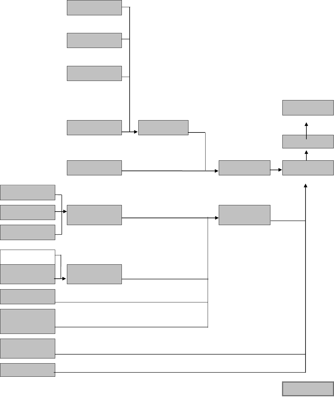
HILDA User Manual – Release 10 57 Last modified: 6/12/11

Figure 4.7: Financial year income model (enumerated person-level)

FY wages and salary

(_wsfes)

Topcoded

[1] Substitute the wave identifier ('a', 'b' ...) for the underscore in variable names.

[2] (= _*p – _*n). In HILDA, negative values are reserved for missing values. Variables

which can legitimately take negative values are supplied in the datasets as two

variables, one positive (suffix 'p') and one negative (suffix 'n'). The result is the

difference.

[3] Shading indicates imputed when missing or when an adult was not interviewed.

Children aged < 15 years old are set to zero on all income measures in the enumerated

person file. Unimputed variables are not supplied in the Enumerated Person file.

[4] Topcode: In the General Release datasets, selected components and sub-totals are

top-coded. To preserve variance, datum equal to or above the threshold have the

weighted mean (weighted by _hhwte) of all values above the threshold substituted for

the actual value. The substituted value will be greater than the threshold. Note that sub-

totals are added and top-coded independently, so for the top-coded cases the sub-total

will not appear to be the result of adding the components.

[5] flag: Imputation flag.

[6] Variable _wsfes is only in wave 10. In waves 1-9 this variable is _wsfei

[**] Child care benefit (CCB) estimate no longer included in benefit income

[***] Only provided on the In-confidence Release files.

flag: _wsfef

FY business income

(=_bifip - _bifin)

Topcoded

flag: _biff

FY investment income

(=_oifinip - _oifinin)

Topcoded

flag: _oifinf

FY disposable income

(=_tifdip-_tifdin)

Topcoded

flag:_tifdif

FY private pensions

(_oifppi)

FY market income

(=_tifmkip - _tifmkin)

Topcoded

flag: _oifppf

flag: _tifmktf

FY estimated taxes

(_txtot)

FY private transfers

(_oifpti)

FY private income

(=_tifpiip - _tifpiin)

Topcoded

FY gross income

(= _tifefp - _tifefn)

Topcoded

flag: _oifptf

flag: _tifpif

flag: _tifeff

Australian Gov’t

pensions

(_bnfpeni)

flag: _bnfpenf

Australian Gov’t

Parenting Payments

(_bnfpari)

Australian Gov’t

income support

payments

(_bnfisi)

FY Australian public

transfers

(_bnfapti)

flag: _bnfparf

Australian Gov’t

allowances

(_bnfalli)

flag: _bnfisf

flag: _bnfaptf

flag: _bnfallf

Estimated family

payments

(_bnffama)

Other non-income

support payments, incl.

Mobility and Carer

Allowances (_bnfonii)

Australian Gov’t non-

income support

payments

(_bnfnisi)

flag: _bnfonif

flag: _bnfnisf

2008-09 Australian

Governement bonus

payments(_bnfobi)

flag: _bnfonf

Other domestic

government benefits

and Australian Gov’t

benefits NEI to classify

(_bnfobi)

flag: _bnfobf

Other regular public

payments (including

scholarships)

(_bnfrpi)

flag: _bnfrpf

Foreign pensions

(_bnffpi)

flag: _bnffpf

FY windfall income

(_oifwfli)

flag: _ oifwflf

HILDA User Manual – Release 10 58 Last modified: 6/12/11

Figure 4.8: Financial year income model (responding-level)

Wages and salary

(_wsfga, _wsfna)

FY wages and salary

(_wsfes)

Topcoded

1] Substitute the wave identifier ('a', 'b' ...) for the underscore in variable

names.

[2] (= _*p – _*n). In HILDA, negative values are reserved for missing values.

Variables which can legitimately take negative values are supplied in the

datasets as two variables, one positive (suffix 'p') and one negative (suffix 'n').

The result is the difference.

[3] Shading indicates imputed when missing (suffix 'i') and vice-versa. For

responding persons the unimputed variables are also supplied in the datasets.

[4] Topcode: In the General Release datasets, selected components and sub-

totals are top-coded. To preserve variance, datum equal to or above the

threshold have the weighted mean (weighted by _hhwtrp) of all values above

the threshold substituted for the actual value. The substituted value will be

greater than the threshold. Note that sub-totals are added and top-coded

independently, so for the top-coded cases the sub-total will not appear to be

the result of adding the components.

[5] flag: Imputation flag.

[6] Variable _wsfes is only in wave 10. In waves1-9 this variable is _wsfei

[*] To avoid double-counting, payments from resident parents are excluded

when windfall income is aggregated to household.

[**] Child care benefit (CCB) estimate no longer included in benefit income.

[***] Only provided on the In-confidence Release files.

Incorporated

business

wages and salary

(_bifiga)

flag: _wsfef

Unincorporated

business income

(_bifuga)

FY business income

(= _bifip - _bifin)

Topcoded

flag: _biff

Interest

(_oifinta)

Rent

(_oifrnta)

FY investment

income

(=_oifinip - _oifinin)

Topcoded

Royalties

(_oifroya)

flag: _oifinf

Dividends from

(_oifdiva)

Dividends from

incorp business

(_bifdiva)

FY disposable

income

(=_tifdip-_tifdin)

Topcoded

flag:_tifdif

Superannuation

(_oifsupa)

FY private pensions

(_oifppi)

FY market income

(=_tifmkip - _tifmkin)

Topcoded

Worker's comp /

accident / sickness

(_oifwkca)

flag: _oifppf

flag: _tifmktf

FY estimated taxes

(_txtot)

Child support

(_oifchs)

Other regular

private

(_oifpria)

FY private transfers

(_oifpti)

FY private income

(=_tifpiip - _tifpiin)

Topcoded

FY gross income

(= _tifefp - _tifefn)

Topcoded

flag: _oifptf

flag: _tifpif

flag: _tifeff

Australian Gov’t

pensions

(_bnfpeni)

flag: _bnfpenf

Australian Gov’t

Parenting Payments

(_bnfpari)

FY Australian Gov’t

income support

payments

(_bnfisi)

FY Australian

public transfers

(_bnfapti)

flag: _bnfparf

Australian Gov’t

allowances

(_bnfalli)

flag: _bnfisf

flag: _bnfaptf

flag: _bnfallf

Estimated family

payments

(_bnffama)

Other non-income

support payments,

incl. Mobility and

Carer Allowances

(_bnfonii)

FY Australian Gov’t

non-income support

payments

(_bnfnisi)

flag: _bnfonif

flag: _bnfnisf

Other domestic

government benefits

and Australian Gov’t

benefits NEI to

classify

(_bnfobi)

flag: _bnfobf

2008-09 Bonus

payments

(_bnfboni)

flag: _bnfbonf

Other regular public

payments (including

scholarships)

(_bnfrpi)

flag: _bnfrpf

Foreign pensions

(_bnffpi)

flag: _bnffpf

HILDA User Manual – Release 10 59 Last modified: 6/12/11

Figure 4.8: (c’td)

Inheritance / Bequests

(_oifinha)

and

From non-household

members

(_oifohha)

Redundancy /

Severance

(_oifrsva)

and

Other irregular

payment

(_oifirra)

FY windfall income

(_oifwfli)

Payments from non-

resident parents

(_oifnpt)

and

Payments from

resident parents

(_oifrpt) [*]

flag: _ oifwflf

Lump sum

superannuation

(_oiflssa)

and

Lump sum workers

compensation

(_oiflswa)

Additional derived income variables are provided in Table 4.15 and Table 4.17, the

latter containing variables directly related to the income imputation. There are

several issues to take note of in Table 4.15:

• Wages and salaries were asked of respondents for their main job, then for

all their other jobs combined. The suffix ‘g’ and ‘e’ refer to gross and

estimated gross incomes – where the respondent didn’t know their gross

income, their after tax income was asked for and this was translated back

into an estimated gross income. The ‘e’ variables will have fewer cases

with missing wages and salaries than the ‘g’ variables, as the ‘e’ variables

include all the known ‘g’ values.

• The variable labels indicate when top-coding has occurred. The actual

value replacing the top-coded value will be the weighted mean of the top-

coded units (see Section 3.12 on Confidentialisation).

• Child support is calculated from the questions asked about the children in

the family formation grid, rather than from the single category listed in the

‘other income’ question in the income section. This is because it is more

likely the respondent would provide a more accurate response to the

detailed questions rather than the broad ‘catch all’ question.

• The components feeding into the ‘windfall’ income are those thought to be

irregular (such as inheritances, redundancies, payments from parents,

lump sum superannuation payouts, lump sum workers compensation

payouts).

• In wave 1, respondents were asked how different their current wage and

salary income was from one year ago. This has been provided in dollar

terms in awsly.

The imputation method and derived variables are discussed in the following sections.

HILDA User Manual – Release 10 - 60 - Last modified: 6/12/2011

Table 4.15: Other derived income variables

Variable Description

Current wages and salaries and current benefits – person-level

_wscg, _wscmg,

_wscog

Current gross wages per week ($), weighted topcode

- All jobs

- Main job

- Other jobs

_bncis, _bncisi,

_bncisf,

Current weekly Gov’t pensions and benefits (pre-imputed, post-imputed, flag),

_bncnis,

_bncnisi,_bncnisf,

Current weekly Gov’t non-income support payments (pre-imputed, post-

imputed, flag)

_bncapu, _bncapui,

_bncapuf

Current weekly Gov’t transfers (pre-imputed, post-imputed, flag)

Financial year income – unimputed variables – person-level

awsly

Gross weekly current wages & salary (from all jobs) one year ago ($)

_wsfg, _oiint,

_oirntp, _oirntn,

_oidiv, _oiroy,

_oidvry, _tifmktp,

_tifmktn, _tifprip,

_tifprin

Financial year income ($):

- gross wages & salary (weighted topcode

)

- interest

- rental income (positive and negative)

- dividends

- royalties

- dividends plus royalties

- market (factor) income (positive and negative, weighted topcode

)

- private income (positive and negative, weighted topcode

)

Current wages and salaries and current benefits – household-level

_hicisi, _hicisf,

_hicnisi, _hicnisf,

_hicapi,_ hicapf

Current weekly Gov’t pensions and benefits (post-imputed, flag),

Current weekly Gov’t non-income support payments (post-imputed, flag),

Current weekly Gov’t transfers (post-imputed, flag)

Financial year income – estimated CCB, FTB A, FTB B, income tax and Medicare levy –

household-level

_hifccb Household Child Care Benefit ($) financial year

_bnccbf1, _bnccbf2,

_bnccbf3

Child Care Benefit ($) for financial year for family number 1, 2 and 3

_bnftaf1, _bnftaf2,

_bnftaf3

Family Tax Benefit Part A ($) for financial year for family number 1, 2 and 3

_bnftbf1, _bnftbf2,

_bnftbf3

Family Tax Benefit Part B ($) for financial year for family number 1, 2 and 3

_bnmatf1, _bnmatf2,

_bnmatf3

Maternity Payments ($) for financial year for family number 1, 2 and 3

_hiffama Australian Gov’t family payments

HILDA User Manual – Release 10 - 61 - Last modified: 6/12/2011

Table 4.15 (c’td)

Variable Description

_txinc, _txmed Financial year taxes ($):

- estimated income tax (weighted topcode

)

- estimated Medicare (weighted topcode

)

Salary sacrifice and non-cash benefit – current and financial year – person level

_sscmrei, _sscorei,

_ssfarei

Whether salary sacrifice was reported in wages and salaries [imputed]

- current main job

- current other jobs

- financial year

_wscmes, _wscoes,

_wsces

Current weekly gross wages & salary including salary sacrifice [imputed]

- current main job

- current other jobs

- financial year

Salary sacrifice and non-cash benefit – current and financial year – household level

jhiwscms, jhisscmf

Household current weekly gross wages & salary including salary sacrifice -

main job (post-imputed, flag)

jhiwscos, jhisscof

Household current weekly gross wages & salary including salary sacrifice -

other jobs (post-imputed, flag)

jhiwsces

Household current weekly gross wages & salary - all jobs ($) [imputed][inc

salary sacrifice]

jhifnb, jhifnbf

Household financial year non-cash benefits (post-imputed, flag)

1. See section on Confidentialisation for explanation of top-coding.

2. Wave 1 only

3. These variables are as calculated from reported wage and salary income and may include salary sacrifice income. They are

consistently measured across waves 1-10.

4.17.2 Imputation Method

The imputation methods used in the HILDA Survey, to varying extents, are:

• Nearest Neighbour Regression method;

• Little and Su method;

• Population Carryover method; and

• Hotdeck method.

The particular combination of methods adopted for the imputation of income data

resulted from a detailed study undertaken by Starick and Watson (2007) and

employs the first three of these four methods.

The imputation steps for each income variable are as follows:

• Step 1 – Carryover of zeros. For non-responding persons (in responding

households), the income amounts are determined to be zero or non-zero

by carrying forward or backward this information from the surrounding

waves with the same probability as that observed in complete cases.

HILDA User Manual – Release 10 - 62 - Last modified: 6/12/2011

• Step 2 – Nearest Neighbour Regression imputation. The predicted values

from a regression model are used to identify a donor from which the

reported value is taken as the imputed value for the recipient. For non-

respondents, a single donor for all income components is used and the

zero or non-zero determination from step 1 is observed.

• Step 3 – Little and Su imputation. This method incorporates (via a

multiplicative model) the trend across waves (column effect), the

recipient’s departure from the trend (row effect), and a residual effect

donated from another respondent with complete income information for

that component (residual effect). Wherever possible, the Little and Su

imputation replaces the Nearest Neighbour Regression imputation. The

zero or non-zero determination from step 1 is observed.

Imputation classes are used for some variables to ensure the donors and recipients

match on a small number of characteristics. Total income is the sum of the imputed

components.

A full description of the imputation process for the income variables is provided by

Hayes and Watson (2009). Appendix 2 provides an extract from this paper which

details the Population Carryover method, Nearest Neighbour Regression method

and Little and Su method.

Table 4.16 shows the percentage of missing cases that were imputed by each

imputation method (for the proportion of cases which are missing, see Table 6.2. The

percentages are summarized across all income variables that have been imputed.

Ideally all records would be imputed by the Little and Su method, however sufficient

information is not always available (especially for non-respondents within responding

households).

With additional waves of income data and improvements to the imputation

methodology, the imputed values will change from Release to Release.

Table 4.16: Percentage of missing cases imputed by imputation method (income), waves 1 to 10

Wave

Imputation method

1 2 3 4 5 6 7 8 9 10

Responding Persons

Nearest Neighbour 10.7 2.1 1.7 1.5 1.5 1.7 1.7 1.1 3.2 7.7

Little & Su 89.3 97.9 98.3 98.3 98.5 98.3 98.3 98.9 96.8 92.3

Enumerated Persons

Nearest Neighbour 59.7 42.5 45.6 44.1 46.1 48.1 48.0 42.2 47.1 53.7

Little & Su 25.6 29.1 30.6 27.8 32.4 33.6 33.6 33.1 35.8 33.0

Carryover 14.8 28.4 23.7 28.1 21.5 18.4 18.4 24.7 17.1 13.2

HILDA User Manual – Release 10 - 63 - Last modified: 6/12/2011

In wave 9, certain stimulus payments were imputed (via the nearest neighbour

method) for those whom receipt of such payments could not be determined from

their financial and family situation. This imputation occurred for:

• the bonus payment for training and learning, the temporary supplement to the

Education Entry Payment, and the farmers hardship bonus (both for

respondents and for non-respondents in responding households); and

• the bonus payment for pensions, seniors, people with disabilities, carers and

veterans (for non-respondents in responding households).

The new questions on salary sacrifice and non-cash benefit variables in wave 10

were imputed. Two methods were used; the nearest neighbour regression was used

to impute the amount of salary sacrificed or the amount of non-cash benefits; and the

nearest neighbour logistic regression method was used to impute whether someone

included these amounts in their report of wages and salaries. This imputation was

undertaken for a person’s main job held currently, other jobs held current, and

together for all jobs held in the last financial year.

4.17.3 Imputed Income Variables

All income imputation was undertaken at the derived variable level, leaving the

original data unchanged. In the main, both the pre-imputed and post-imputed

variables are available in the datasets, along with an imputation flag, so that it is

easy to choose between using the pre-imputed data or the post-imputed data.

An overview of the pre- and post-imputed income variables is provided in Table 4.17.

Table 4.17: Imputed income variables

Pre-imputed Post-imputed Flag

Responding person file

Current income

Wages and salaries – all jobs _wsce _wscei _wscef

Wages and salaries – main job _wscme _wscmei _wscmef

Wages and salaries – other jobs _wscoe _wscoei _wscoef

Salary sacrifice – main job

_sscm _sscmi _sscmf

Salary sacrifice – other jobs

_ssco _sscoi _sscof

Non-cash benefits – main job

_nbcm _nbcmi _nbcmf

Non-cash benefits – other jobs

_nbco _nbcoi _nbcof

Australian Gov’t pension _bncpen _bncpeni _bncpenf

Australian Gov’t parenting

payment

_bncpar _bncpari _bncparf

Australian Gov’t allowances _bncall _bncalli _bncallf

Non-income support other than

family payment

_bnconi _bnconii _bnconif

HILDA User Manual – Release 10 - 64 - Last modified: 6/12/2011

Table 4.17: (c’td)

Pre-imputed Post-imputed Flag

Other domestic gov’t benefits and

Australian Gov’t NEI to classify

_bncob

_bncobi _bncobf

Financial year income

Wages and salaries _wsfe _wsfei _wsfef

Salary sacrifice

_ssfa _ssfai _ssfaf

Non-cash benefits

_nbfa _nbfai _nbfaf

Australian Gov’t pension _bnfpen _bnfpeni _bnfpenf

Australian Gov’t parenting

payment

_bnfpar _bnfpari _bnfparf

Australian Gov’t allowances _bnfall _bnfalli _bnfallf

Australian Governments Bonus

payments (2008-09)

_bnfbon _bnfboni _ bnfbonf

Non-income support other than

family payment

_bnfoni _bnfonii _bnfonif

Other regular public payments _bnfrp _bnfrpi _bnfrpf

Other domestic gov’t benefits and

Australian Gov’t NEI to classify

_bnfob

_bnfobi _bnfobf

Foreign gov’t pensions _bnffp _bnffpi _bnffpf

Business income _bifn, _bifp _bifin, _bifip _biff

Investments _oifinvn, _oifinvp _oifinin, _oifinip _oifinf

Private pensions _oifpp _oifppi _oifppf

Private transfers _oifpt _oifpti _oifptf

Total FY income

Not provided _tifefn, _tifefp _tifeff

Windfall income _oifwfl _oifwfli _oifwflf

Enumerated person file

Current income

Wages and salaries – all jobs - _wscei _wscef

Wages and salaries – main job - _wscmei _wscmef

Wages and salaries – other jobs - _wscoei _wscoef

Salary sacrifice – main job

- _sscmi _sscmf

Salary sacrifice – other jobs

- _sscoi _sscof

Non-cash benefits – main job

- _nbcmi _nbcmf

Non-cash benefits – other jobs

- _nbcoi _nbcof

Australian Gov’t pension - _bncpeni _bncpenf

Australian Gov’t parenting

payment

- _bncpari _bncparf

HILDA User Manual – Release 10 - 65 - Last modified: 6/12/2011

Table 4.17: (c’td)

Australian Gov’t allowances - _bncalli _bncallf

Non-income support other than

family payment

- _bnconii _bnconif

Other domestic gov’t benefits and

Australian Gov’t NEI to classify

- _bncobi _bncobf

Financial year income

Wages and salaries - _wsfei _wsfef

Salary sacrifice

- _ssfai _ssfaf

Non-cash benefits

- _nbfai _nbfaf

Australian Gov’t pension - _bnfpeni _bnfpenf

Australian Gov’t parenting

payment

- _bnfpari _bnfparf

Australian Gov’t allowances - _bnfalli _bnfallf

Australian Government Bonus

payments (2008-09)

- _bnfboni _ bnfbonf

Non-income support other than

family payment

- _bnfonii _bnfonif

Other regular public payments - _bnfrbi _bnfrbf

Other domestic gov’t benefits and

Australian Gov’t NEI to classify

- _bnfobi _bnfobf

Foreign gov’t pensions - _bnffpi _bnffpf

Business income - _bifin, _bifip _biff

Investments - _oifinin, _oifinip _oifinf

Private pensions - _oifppi _oifppf

Private transfers - _oifpti _oifptf

Total FY income

- _tifefn, _tifefp _tifeff

Windfall income - _oifwfli _oifwflf

Household file

Current income

Wages and salaries – all jobs - _hiwscei _hiwscef

Wages and salaries – main job - _hiwscmi _hiwscmf

Wages and salaries – other jobs - _hiwscoi _hiwscof

Australian Gov’t pension - _hicpeni _hicpenf

Australian Gov’t parenting

payment

- _hicpari _hicparf

Australian Gov’t allowances - _hicalli _hicallf

HILDA User Manual – Release 10 - 66 - Last modified: 6/12/2011

Table 4.17: (c’td)

Non-income support other than

family payment

- _hiconii _hiconif

Other domestic gov’t benefits and

Australian Gov’t NEI to classify

- _hicobi _hicobf

Financial year income

Wages and salaries - _hiwsfei _hiwsfef

Australian Gov’t pension - _hifpeni _hifpenf

Australian Gov’t parenting

payment

- _hifpari _hifparf

Australian Gov’t allowances - _hifalli _hifallf

Australian Government Bonus

payments (2008-09)

- _hifboni _hifbonf

Non-income support other than

family payment

- _hifonii _hifonif

Other regular public payments - _hifrpi _hifrpf

Other domestic gov’t benefits and

Australian Gov’t NEI to classify

- _hifobi _hifobf

Foreign govt pensions - _hiffpi _hiffpf

Business income - _hibifin, _hibifip _hibiff

Investments - _hifinin, _hifinip _hifinf

Private pensions - _hifppi _hifppf

Private transfers - _hifpti _hifptf

Total FY income - _hifefn, _hifefp _hifeff

Windfall income - _hifwfli _hifwflf

1. In wave 10 only.

2. In wave 9 only.

3. The following variables use total person financial year income (_tifefn, _tifefp) in their calculations: income tax (_txinc), and

Medicare (_txmed). Use _tifeff as imputation flag for these variables.

4.18 Wealth (Special Topic in Waves 2, 6 and 10)

4.18.1 Wealth Model

In waves 2, 6 and 10 a special wealth module was incorporated into the

questionnaires. The Household Questionnaire contained the majority of the wealth

questions and we endeavoured to ask these of the person knowing the most about

the household finances. These questions covered the following topics:

• Cash and equity investments, trust funds, life insurance;

• Home and other property assets and debts;

• Business assets and debts;

HILDA User Manual – Release 10 - 67 - Last modified: 6/12/2011

• Children’s bank accounts;

• Collectables and vehicles, and

• Overdue household bills (in wave 6 only

Also, each respondent was asked some questions about their personal wealth in the

Person Questionnaire, including:

• Bank accounts and credit card debt;

• Superannuation;

• HECS debt; and

• Other personal debts

Figure 4.9 shows how the wealth components are combined together to form the

total household wealth. The boxes with the broken lines highlight the variables that

come from the Person Questionnaire. From Release 6, the imputation for non-

respondents has been conducted at the wealth component level, so the household-

level components are the sum of all persons in the household.

That is, bank accounts of people in the household aged under 15.

Overdue household bills were explicitly asked for in wave 6. It was assumed that this was captured

in the ‘any other debt’ question asked in wave 2 (though perhaps not well).

In wave 6, these other personal debts were asked for at a more disaggregated level and overdue

personal bills were also explicitly asked for.

For Release 2 to 5, please note that the imputation for non-respondents was only conducted at the

total assets and debts level. As a result the household-level components that summed these person-

level components was just the sum of responding persons only. This will explain some of the

differences observed for these variables between releases.

HILDA User Manual – Release 10 - 68 - Last modified: 6/12/2011

Figure 4.9: Wealth model (household-level)

Joint bank accounts

(_hwjbani, flag _hwjbanf)

[1] Only the names of the imputed variables and their flags have been provided in this

figure.

[2] Variables in solid boxes in first column are derived from the Household

Questionnaire. Variables in the broken line boxes are household level variables

derived by summing the equivalent components for adults in the household.

[3] Item non-response in the HQ has been imputed by linking household longitudinally

where possible.

[4] Item non-response for respondents, together with unit and wave non-response for

non-respondents in households where there was at least one respondent, has been

imputed at the component level.

[5] Shading indicates imputed when missing (suffix ‘I’).

[6] (=_*p - _*n). In HILDA, negative values are reserved for missing values. Variables

which can legitimately take negative values are supplied in the dataset as two

variables, one positive (suffix ‘p’) and one negative (suffix ‘n’). The result is the

difference.

[7] Net equity variables not shown on this diagram have been calculated for business

(=_hwbusep-_hwbusen), home (_hwhmeqp-_hwhmeqn), other property (_hwopeqp-

_hwopeqn) and total property (_hwtpeqp-_hwtpeqn).

[*] Other personal debts in wave 6 were asked by type and include overdue personal

bills.

Own bank accounts

(_hwobani, flag _hwobanf)

Bank accounts

(_hwtbani, flag

_hwtbanf)

Children’s bank

accounts

(_hwcbani, flag _hwcbanf)

Superannuation –

retirees

(_hwsupri, flag _hwsuprf)

Superannuation

(_hwsupei, flag

_hwsupef)

Superannuation –

non-retirees

(_hwsupwi, flag

_hwsupwf)

Cash investments

(_hwcaini, flag _hwcainf)

Equity investments

(_hweqini, flag _hweqinf)

Financial assets

(_hwfini, flag _hwfinf)

Trust funds

(_hwtrusi, flag _hwtrusf)

Life insurance

(_hwinsui, flag _hwinsuf)

Total assets

(_hwassei,

flag _hwassef)

Home asset

(_hwhmvai, flag

_hwhmvaf)

Property asset

(_hwtpvi, flag _hwtpvf)

Other property assets

(_hwopvai, flag _hwopvaf)

Business assets

(_hwbusvi, flag _hwbusvf)

Non-financial assets

(_hwnfii, flag _hwnfif)

Collectibles

(_hwcolli, flag _hwcollf)

Vehicles

(_hwvechi, flag _hwvechf)

Net worth

(=_hwnwip -

_hwnwin, flag

_hwnwf)

Joint credit cards

(_hwjccdi, flag _hwjccdf)

Credit card debt

(_hwccdti, flag

_hwccdtf)

Own credit cards

(_hwoccdi, flag _hwoccdf)

HECS debt

(_hwhecdi, flag _hwhecdf)

Other personal debt *

(_hwothdi, flag _hwothdf)

Total debts

(_hwdebti, flag

_hwdebtf)

Business debt

(_hwbusdi, flag _hwbusdf)

Home debt

(_hwhmdti, flag _hwhmdtf)

Property debt

(_hwtpdi, flag _hwtpdf)

Other property debt

(_hwopdti, flag _hwopdtf)

Overdue HH bills

[wave 6]

(_hwobdti, flag _hwobdtf)

HILDA User Manual – Release 10 - 69 - Last modified: 6/12/2011

Several equity variables (assets less debts) not described in the previous figure are

provided on the household file. These are business equity, home equity, other

property equity, and total property equity. These variables, together with the

unimputed versions of the sub-totals described in Figure 4.9 are provided in Table

4.18 (variables relating directly to the wealth imputation are provided later in Table

4.21).

Table 4.18: Other derived wealth variables at household-level

Pre-imputed Post-imputed Imputation flag

Business equity (weighted topcode) _hwbusep,

_hwbusen

_hwbeip,

_hwbein

_hwbef

Home equity (weighted topcode) _hwhmeqp,

_hwhmeqn

_hwhmeip,

_hwhmein

_hwhmef

Other property equity (weighted topcode) _hwopeqp,

_hwopeqn

_hwopeip,

_hwopein

_hwopef

Total property equity (weighted topcode) _hwtpeqp,

_hwtpeqn

_hwtpeip,

_hwtpein

_hwtpef

Total property value (weighted topcode) _hwtpval

Home loans

- from financial institution

- from other source (friend, relative, etc)

- secured against property

_hwhmhl,

_hwhmol,

_hwhmeql

Total property debt (weighted topcode) _hwtpdt

Total credit card debt _hwccdt

Retiree’s superannuation _hwsuprt

Total superannuation (weighted topcode) _hwsuper

Total bank accounts (weighted topcode) _hwtbank

Household financial assets (weighted topcode) _hwfin

Household non-financial assets (weighted

topcode)

_hwnfin

4.18.2 Imputation Method

The imputation method adopted for the wealth data takes advantage of three

observation points (waves 2, 6 and 10).

• Step 1 – Create a longitudinal household identifier. For variables imputed

at the household-level, households are linked longitudinally if they had

common membership and any additional household members were

A summary of the steps in the imputation

process is provided below:

For Release 2 through to 5, the wealth imputation for wave 2 used the Nearest Neighbour

Regression method (see Watson, 2004a for more details).

HILDA User Manual – Release 10 - 70 - Last modified: 6/12/2011

children (defined for this purpose to be under 18 years of age) and any

missing household members were children or deceased.

• Step 2 – Nearest Neighbour Regression imputation of zeros. The

predicted values from a regression model are used to identify a donor from

which to flag zero or non-zero imputes for the recipient. This is essentially

a filter process to decide whether the case has the asset or debt.

• Step 3 – Nearest Neighbour Regression imputation of non-zero amounts.

The predicted values from a regression model are used to identify a donor

from which the reported value is taken as the imputed value for the

recipient. The models and donor pools are restricted to cases with non-

zero amounts.

• Step 4 – Little and Su imputation. This method incorporates (via a

multiplicative model) the trend across waves (column effect), the

recipient’s departure from the trend (row effect), and a residual effect

donated from another case with complete wealth information for that

component (residual effect). Wherever possible, the Little and Su

imputation replaces the Nearest Neighbour Regression imputation. The

zero or non-zero determination from step 2 is observed.

Imputation classes were used for some variables to ensure the donors and recipients

match on a small number of characteristics (typically wealth bands and filter

variables).

Note that the household-level wealth variable for home value was collected in all

waves and has been imputed via the same approach outlined above. _hhlink is an

indicator variable showing whether a household was linked to another household in

the next wave for the purposes of imputing home value.

A detailed description of the imputation process for wealth variables is provided by

Hayes and Watson (2009). Appendix 2 provides an extract from this paper which

details the Nearest Neighbour Regression method and Little and Su method.

Table 4.19 and Table 4.20 show the percentage of missing cases that were imputed

by each imputation method.

In the first table the percentages are summarized

across all wealth variables that have been imputed. As with income it is preferable to

have all records imputed by the Little and Su method but, with only three waves of

wealth data, sufficient information was not always available. Non-respondents in the

enumerated person group were less likely to be imputed by the Little and Su method

(for similar reasons as in income imputation) and any households not linked between

waves were imputed via the nearest neighbour regression method.

Table 4.20 shows a much higher percentage of records imputed via the Little and Su

method for home value due to better household linking between consecutive waves

(rather than the four-wave difference experienced with the imputation of other wealth

variables).

bhwlink is an indicator variable for whether the wave 2 household could be linked to a wave 6

household.

For the proportion of cases which are missing, see Table 6.6 and Table 6.7.

HILDA User Manual – Release 10 - 71 - Last modified: 6/12/2011

Table 4.19: Percentage of missing cases imputed by imputation method (wealth), waves 2, 6, and

Imputation Method Wave 2 Wave 6 Wave 10

Person level wealth items (responding persons)

Nearest Neighbour 48.2 46.4 57.0

Little & Su 51.8 53.6 43.0

Person level wealth items (enumerated persons)

Nearest Neighbour 76.8 69.9 72.4

Little & Su 23.2 30.1 27.6

Household level wealth items

Nearest Neighbour 39.6 34.6 43.7

Little & Su 60.4 65.4 56.3

Table 4.20: Percentage of missing cases imputed by imputation method (home value), waves 1

to 10

Wave

Imputation Method 1 2 3 4 5 6 7 8 9 10

Home value (households)

Nearest Neighbour 26.6 5.3 15.6 14.4 14.7 12.8 11.6 7.9 11.9 27.4

Little & Su 73.4 94.7 84.4 85.6 85.4 87.2 88.4 92.1 88.1 72.6

Number imputed 312 378 269 187 157 196 121 138 168 237

4.18.3 Imputed Wealth Variables

Table 4.21 outlines the imputed wealth variables included on the wave 2 and 6 files.

Further, as mentioned earlier, home value, _hsvalue, has been imputed in all waves

(_hsvalui) and the imputation flag provided (_hsvaluf). _hsvalue differs from

_hwhmval in that it is the total value of the home, whereas _hwhmval is the share

owned by the household members (which is just collected in waves 2 and 6).

HILDA User Manual – Release 10 - 72 - Last modified: 6/12/2011

Table 4.21: Imputed wealth variables

Pre-imputed Post-imputed Flag

Responding person file

Assets

Joint bank accounts _pwjbank _pwjbani _pwjbanf

Own bank accounts _pwobank _pwobani _pwobanf

Superannuation – retirees _pwsuprt _pwsupri _pwsuprf

Superannuation – non-retirees _pwsupwk _pwsupwi _pwsupwf

Debts

HECS debt _pwhecdt _pwhecdi _pwhecdf

Joint credit cards _pwjccdt _pwjccdi _pwjccdf

Own credit cards _pwoccdt _pwoccdi _pwoccdf

Other personal debt _pwothdt _pwothdi _pwothdf

Enumerated person file

Assets

Joint bank accounts - _pwjbani _pwjbanf

Own bank accounts - _pwobani _pwobanf

Superannuation – retirees - _pwsupri _pwsuprf

Superannuation – non-retirees - _pwsupwi _pwsupwf

Debts

HECS debt - _pwhecdi _pwhecdf

Joint credit cards - _pwjccdi _pwjccdf

Own credit cards - _pwoccdi _pwoccdf

Other personal debt - _pwothdi _pwothdf

Household file

Assets

Joint bank accounts _hwjbank _hwjbani _hwjbanf

Own bank accounts _hwobank _hwobani _hwobanf

Children’s bank accounts _hwcbank _hwcbani _hwcbanf

Superannuation – retirees _hwsuprt _hwsupri _hwsuprf

Superannuation – non-

retirees

_hwsupwk _hwsupwi _hwsupwf

Business assets _hwbusva _hwbusvi _hwbusvf

Cash investment _hwcain _hwcaini _hwcainf

Equity investment _hweqinv _hweqini _hweqinf

Collectibles _hwcoll _hwcolli _hwcollf

Home asset _hwhmval _hwhmvai _hwhmvaf

Other property assets _hwopval _hwopvai _hwopvaf

Life insurance _hwinsur _hwinsui _hwinsuf

Trust funds _hwtrust _hwtrusi

_hwtrusf

Vehicles value _hwvech _hwvechi _hwvechf

Total household assets

_hwasset _hwassei _hwassef

HILDA User Manual – Release 10 - 73 - Last modified: 6/12/2011

Table 4.21: (c’td)

Pre-imputed Post-imputed Flag

Debts

HECS debt _hwhecdt _hwhecdi _hwhecdf

Joint credit cards _hwjccdt _hwjccdi _hwjccdf

Own credit cards _hwoccdt _hwoccdi _hwoccdf

Other personal debt _hwothdt _hwothdi _hwothdf

Business debt _hwbusdt _hwbusdi _hwbusdf

Home debt _hwhmdt _hwhmdti _hwhmdtf

Other property debt _hwopdt _hwopdti _hwopdtf

Overdue household bills

_hwobdt _hwobdti _hwobdtf

Total household debts _hwdebt _hwdebti _hwdebtf

Net worth _hwnetwp, _hwnetwn _hwnwip, _hwnwin _hwnwf

1. Variable not in wave 1.

4.19 Expenditure

In every wave, HILDA collects housing expenditures (rent and mortgage

repayments) in the Household Questionnaire. The household expenditure on

groceries, food and meals eaten outside were collected in the Household

Questionnaire for wave 1, 3, 4, and 5. Household expenditure on a wide range of

goods and services were first collected in the wave 5 Self-Completion Questionnaire.

The list of items collected was expanded to include consumer durables from wave 6.

While the person in the household responsible for the household bills was asked to

complete the household-level expenditure questions in the SCQ, sometimes more

than one person in a household provided answers. The variables with the prefix _hx

average the responses across all individuals who provided a response to these

expenditure questions (the responses from dependent students who stated they are

not responsible for the household bills are excluded).

4.19.1 Imputation Method

The expenditure variables were imputed for the first time in Release 8 and were

extended to include the imputation of child care costs for Release 9. A summary of

the steps in the imputation process is provided below:

• Step 1 – Create a longitudinal household identifier. For variables imputed

at the household-level, households are linked longitudinally if they had

common membership.

For each of the _hx pre-imputed variables listed in

Deaths and births, for the purposes of

expenditure imputation, are counted as a membership change.

Table 4.23, corresponding _px variables are provided,

which are the derived annualised response for each person who provided a response to these questions. Most

users will use the _hx variables.

_hxylink is an indicator variable for whether a household was linked to another household in the

next wave for the purposes of imputing expenditure.

HILDA User Manual – Release 10 - 74 - Last modified: 6/12/2011

• Step 2 – Identify lumpy expenditure items. Some items (such as cars,

white goods, etc) would not be purchased each year, so need to be

treated differently in the imputation process.

• Step 3 – Carryover zeros. The population carryover method is used to

determine zero and non-zero expenditure flags for non-lumpy expenditure

items prior to any other imputation. Lumpy expenditure items were

excluded from this step.

• Step 4 – Nearest Neighbour Regression imputation of zeros. The

predicted values from a regression model are used to identify a donor from

which to flag zero or non-zero imputes for the recipient. This is essentially

a filter process to decide whether the case has the expense or not.

• Step 5 – Nearest Neighbour Regression imputation of non-zero amounts.

The predicted values from a regression model are used to identify a donor

from which the reported value is taken as the imputed value for the

recipient. The models and donor pools are restricted to cases with non-

zero amounts. For households without any expenditure data reported in

the SCQ, a single donor for all expenditure variables collected in the SCQ

was used.

• Step 6 – Little and Su imputation. This method incorporates (via a

multiplicative model) the trend across waves (column effect), the

recipient’s departure from the trend (row effect), and a residual effect

donated from another case with complete expenditure information for that

component (residual effect). Only cases that have been enumerated in

more than one wave, longitudinally linked, and have at least one wave of

non-zero data available can be imputed via this method. For the lumpy

expenditure items, the donors selected had to have the same zero pattern

for the non-missing waves as the recipients. Wherever possible, the Little

and Su imputation replaces the Nearest Neighbour Regression imputation.

The zero or non-zero determination from steps 3 and 4 is observed.

Imputation classes were used for some variables to ensure the donors and recipients

match on a small number of characteristics (typically equivalised household

disposable income bands and the age group of the highest income earner were

used).

A full description of the imputation process for the expenditure variables is provided

by Sun (2010). Appendix 2 provides an extract from Hayes and Watson (2009) which

details the Nearest Neighbour Regression method, the Little and Su method and the

Population Carryover method.

Table 4.22 shows the percentage of missing cases that were imputed by each

imputation method.

For the proportion of cases which are missing, see

Ideally all the records should be imputed by a longitudinal

imputation method, such as the Little and Su method or the Carryover method. The

households which cannot be linked between waves were imputed by the Nearest

Neighbour Regression method regardless of their situation. For the housing

expenditure variables (rent payment, mortgage repayment and second mortgage

Table 6.10.

HILDA User Manual – Release 10 - 75 - Last modified: 6/12/2011

repayment), which have been collected in all waves so far, the majority of cases

were imputed by the Little and Su method. For the expenditure items collected from

wave 6 onwards where we have fewer waves of data available, more than half of the

cases were imputed by the Nearest Neighbour Regression method

Table 4.22: Percentage of missing cases imputed by imputation method (expenditure), waves 1

to 10

Wave

Imputation method

1 2 3 4 5 6 7 8 9 10

Housing and work-related childcare expenditure variables (collected in all waves Household

Questionnaire)

Nearest Neighbour 45.2 13.6 23.2 22.9 14.4 25.6 16.9 21.7 24.5 48.4

Little & Su 47.0 71.4 69.7 72.4 76.8 69.9 74.4 74.7 63.5 41.8

Carryover 7.8 15.0 7.1 4.7 8.8 4.5 8.7 3.6 12.0 9.8

Non-work-related childcare expenditure variables (collected in the Household Questionnaire from

wave 2)

Nearest Neighbour - 61.1 40.0 50.0 72.7 75.0 57.1 66.7 57.4 73.7

Little & Su - 25.0 20.0 38.8 27.2 25.0 38.1 23.8 24.5 26.3

Carryover - 13.9 40.0 11.1 0.0 0.0 4.8 9.5 18.1 0.0

Weekly household expenditure variables (collected in wave 1, 3, 4, and 5 Household

Questionnaire)

Nearest Neighbour 56.2 - 27.6 23.3 35.6 - - - - -

Little & Su 42.8 - 65.4 70.2 56.6 - - - - -

Carryover 1.0 - 7.4 6.5 7.8 - - - - -

Annualised household expenditure variables (collected in the Self-Completion Questionnaire from

wave 5)

Nearest Neighbour - - - - 55.1 38.6 34.9 36.6 38.2 54.3

Little & Su - - - - 34.6 43.9 48.6 46.7 45.8 36.0

Carryover - - - - 10.3 17.5 16.5 16.7 16.0 9.7

Annualised household expenditure variables (collected in the Self-Completion Questionnaire from

wave 6)

Nearest

Neighbour

- - - - -

61.9 46.1 46.6 47.9 65.1

Little & Su - - - - - 32.0 43.9 43.9 42.3 29.6

Carryover - - - - - 6.1 10.0 9.5 9.8 5.3

4.19.2 Imputed Household Expenditure Variables

All expenditure imputation was undertaken at the household level. Both the pre- and

post-imputed variables are available in the datasets, along with an imputation flag.

Table 4.23 provides an overview of the pre- and post-imputed expenditure variables

and the waves in which they are available.

HILDA User Manual – Release 10 - 76 - Last modified: 6/12/2011

Table 4.23: Imputed household expenditure variables

Wave Pre-imputed

Post-imputed Flag

Usual payments/repayments per month (Collected in the HQ)

Rent 1 - 10 _hsrnt _hsrnti _hsrntfg

First mortgage 1 - 10 _hsmg _hsmgi _hsmgfg

Second mortgage 1 - 10 _hssl _hssli _hsslfg

Weekly household expenditure (Collected in the HQ)

All groceries 1, 3 - 5 _xpgroc _xpgroci _xpgrocf

Groceries for food and drink

1, 3 - 5

_xpfood _xpfoodi _xpfoodf

Meals eaten outside

1, 3 - 5

_xposml _xposmli _xposmlf

Annualized household expenditure (Collected in the SCQ)

Groceries 5 – 10 _hxygroc _hxygrci _hxygrcf

Alcohol 5 – 10 _hxyalc _hxyalci _hxyalcf

Cigarettes and tobacco 5 – 10 _hxycig _hxycigi _hxycigf

Public transport and taxis 5 – 10 _hxypubt _hxypbti _hxypbtf

Meals eaten out 5 – 10 _hxymeal _hxymli _hxymlf

Leisure activities 5 _hxyhsge _hxyhsgi _hxyhsgf

Motor vehicle fuel 5 – 10 _hxymvf _hxymvfi _hxymvff

Men's clothing and footwear 6 – 10 _hxymcf _hxymcfi _hxymcff

Women's clothing and footwear 6 – 10 _hxywcf _hxywcfi _hxywcff

Children's clothing and footwear 6 – 10 _hxyccf _hxyccfi _hxyccff

Clothing and footwear 5 _hxyclth _hxyclti _hxycltf

Telephone rent and calls 5 _hxytel _hxytli _hxytlf

Telephone rent and calls, internet

charges 6 – 10

_hxyteli _hxytlii _hxytlif

Holidays and holiday travel costs 5 – 10 _hxyhol _hxyholi _hxyholf

Private health insurance 5 – 10 _hxyphi _hxyphii _hxyphif

Other insurances 6 – 10 _hxyoi _hxyoii _hxyoif

Fees paid to health practitioner 6 – 10 _hxyhltp _hxyhlpi _hxyhlpf

Medicines, prescriptions and

pharmaceuticals 6 – 10

_hxyphrm _hxyphmi _hxyphmf

HILDA User Manual – Release 10 - 77 - Last modified: 6/12/2011

Table 4.23: (c’td)

Wave Pre-imputed

Post-imputed Flag

Health care 5 _hxyhlth _hxyhthi _hxyhthf

Electricity bills 5 _hxyelec _hxyelei _hxyelef

Gas bills 5 _hxygas _hxygasi _hxygasf

Other heating fuel 5 _hxyohf _hxyohfi _hxyohff

Electricity, gas bills and other heating fuel 6 – 10 _hxyutil _hxyutli _hxyutlf

Repairs, renovation and maintenance to

home 5 – 10

_hxyhmrn _hxyhmri _hxyhmrf

Motor vehicle repairs and maintenance 5 – 10 _hxymvr _hxymvri _hxymvrf

Education fees 5 – 10 _hxyeduc _hxyedci _hxyedcf

Buying brand new vehicles 6 – 10 _hxyncar _hxyncri _hxyncrf

Buying used vehicles 6 – 10 _hxyucar _hxyucri _hxyucrf

Computers and related services 6 – 10 _hxycomp _hxycmpi _hxycmpf

Audio visual equipment 6 – 10 _hxytvav _hxytvi _hxytvf

Household appliance 6 – 10 _hxywg _hxywgi _hxywgf

Furniture 6 – 10 _hxyfurn _hxyfrni _hxyfrnf

1. The household-level responses provided by each person in the household responsible for household expenditure are

provided in equivalent variables to the pre-imputed household expenditure variables from the SCQ (_hx is replaced by _xp

to give variables _xpgroc to _xpyfurn). Most users will use the _hx variables.

4.20 Weights

4.20.1 Cross-Sectional Weights

Wave 1

In wave 1, we essentially had a complex cross-sectional survey. The initial (or

design) weights are derived from the probability of selecting the households into the

sample. These household weights are initially adjusted according to information

collected about all selected households (both responding and non-responding) and

further adjusted so that weighted household estimates from the HILDA Survey match

several known household-level benchmarks.

The person-level weights are based on the household-level weights, with

adjustments made based on information collected about all the people listed in the

responding households. These weights are also adjusted to ensure that the weighted

person estimates match several known person-level benchmarks.

More information about the weighting procedure can be found in Watson and Fry

(2002). See the section below for a description of the benchmarks as these have

been modified after Release 1.

HILDA User Manual – Release 10 - 78 - Last modified: 6/12/2011

Wave 2 onwards

From wave 2 onwards, the ‘selection’ of the sample is dependent on the wave 1

responding sample and the household and individual attrition after wave 1. The

cross-sectional weights for wave 2 onwards opportunistically include temporary

members into the sample (i.e., those people who are part of the sample only

because they currently live with a continuing sample member). The underlying

probability of selection for these households is amended to account for the various

pathways from wave 1 into the relevant wave household. Following this, non-

response adjustments are made which require within-sample modelling of non-

response probabilities and benchmarking to known population estimates at both the

household and person level.

The weighting process for wave 2 onwards is detailed in Watson (2004b).

4.20.2 Longitudinal Weights

See the

section below for a description of the benchmarks as these have been modified after

Release 2.

By comparison, the construction of the longitudinal weights is more straightforward

and only include an adjustment for attrition and benchmarking back to the initial

wave characteristics. The longitudinal weights are described in Watson (2004b) but

see the following section for a description of the benchmarks used.

We have provided longitudinal weights for the balanced panel of responding persons

or enumerated persons from every wave to every other wave and for the balanced

panel of any combination of a pair of waves. These weights adjust for attrition from

the initial wave and are benchmarked back to the key characteristics of the initial

wave. For instance if you were interested in a panel of respondents from waves 2

through 6, the weight provided for this panel would adjust for attrition from the

balanced panel from wave 2 to 6 and would ensure key characteristics of the wave 2

population are matched.

4.20.3 Benchmarks

The benchmarks used in the weighting process are listed in Table 4.24

• The household and enumerated person weights are determined at the

same time. This is known as integrated weighting. The weights are

adjusted to the household benchmarks at the same time as they are

adjusted to the enumerated person benchmarks. The household weight

will be the same as the enumerated weight for each person in the

. The

changes made to the benchmarking process originally documented in Watson

(2004b) include:

While this paper is written in relation to the wave 2 weighting, the process in later waves follows the

same methodology.

We thank the Demography Section and the Labour Force Estimates team from the Australian

Bureau of Statistics for the provision of the benchmarks used in the weighting process.

HILDA User Manual – Release 10 - 79 - Last modified: 6/12/2011

household, resulting in identical estimates where the same concept can

be determined from the two files.

• Due to the demands placed on the weights through the integrated

weighting process, some of the benchmarks used have been simplified.

• Following some concerns about the representativeness of the sample,

additional benchmarks on marital status and household composition have

been included.

• The person benchmarks for State, part of State, sex and age are from the

Estimated Residential Population figures produced by the ABS based on

the 2001 Census and the 2006 Census, updated for births, deaths,

immigration, emigration and interstate migration. The household

benchmarks are derived from these person benchmarks by the ABS.

• The person benchmarks for labour force status and marital status come

from the ABS Labour Force Survey.

The person benchmarks for household composition are derived from the

household benchmarks.

• The very remote parts of New South Wales, Queensland, South Australia,

Western Australia and the Northern Territory have been excluded from the

benchmarks, which is in line with the practice adopted in similar large-

scale surveys run by the ABS. As a result, a small number of cases may

have zero weights.

Note also that the benchmarks exclude people living in non-private dwellings, so

people that move into these dwellings after wave 1 are given zero cross-sectional

weights.

For example, the number of people living in a household with two people can be derived by two

methods. Firstly, this can be calculated from the household file by estimating the number of two

person households and multiplying by two. Secondly, it can be estimated from the enumerated file by

summing the weights of people living in two person households.

An occupation benchmark was included from Release 4 to 6, but this was later removed following

concerns about the occupation coding as outlined by Watson and Summerfield (2009).

Due to updates to the household propensities used by the ABS to create the household

benchmarks, the total number of households based on the 2006 Census is quite different from that

based on the 2001 Census. For example, the number of households in Australia in September 2001

based on the 2001 Census was 7.43 million, whereas the corresponding number based on the 2006

Census was 7.32 million. In order to minimise the impact on our estimates caused by changes to the

benchmarks, an incremental combination of the two sets of household benchmarks was taken.

This stemmed from a change in the benchmarks available from the ABS to align with the

remoteness area classification rather than a ‘sparsely settled’ definition.

HILDA User Manual – Release 10 - 80 - Last modified: 6/12/2011

Table 4.24: Benchmarks used in weighting

Household weights

Enumerated person

weights

Responding person

weights

Cross-sectional

weights

• Number of adults by

number of children

• State by part of

State

Determined jointly with

enumerated person

weights

• Sex by broad age

• State by part of

State

• Labour force status

• Marital status

Determined jointly with

household weights

• Sex by broad age

• State by part of State

• State by labour force

status

• Marital status

• Household

composition (number

of adults and

children)

Longitudinal weights Not applicable

• Sex by broad age

• State by part of

State

• Labour force status

• Marital status

• Household

composition

(number of adults

and children)

• Sex by broad age

• State by part of State

• State by labour force

status

• Marital status

• Household

composition (number

of adults and

children)

4.20.4 Replicate Weights

Replicate weights have been provided for users to calculate standard errors that take

into account the complex sample design of the HILDA Survey. These weights can be

used by the SAS GREGWT macro, the STATA ‘svy jackknife’ commands (more

detail is provided below in the section on Calculating Standard Errors), or you can

write your own routine to use these weights. Weights for 45 replicate groups are

provided.

4.20.5 Weights Provided on the Data Files

Table 4.25 provides a list of the weights provided on the data files together with a

description of those weights. The longitudinal weights provided on the enumerated

and responding person files are the ones you are most likely to use, though other

longitudinal weights are provided on the Longitudinal Weights File.

Irrespective of the modifications made in how the weights are constructed, some

changes are expected to the weights with each new release. There are three

reasons for this. Firstly, corrections may be made to age and sex variables when

these are confirmed with individuals in subsequent wave interviews. Secondly, the

benchmarks are updated from time to time. Thirdly, duplicate or excluded people in

the sample may be identified after the release (very occasionally).

HILDA User Manual – Release 10 - 81 - Last modified: 6/12/2011

Table 4.25: Weights

File Weights Description

Household File _hhwth The household weight is the cross-section population weight for all

households responding in the relevant wave. Note the sum of these

household weights for wave 1 is approximately 7.4 million.

_hhwths This is the cross-section household population weight rescaled to

the sum of the sample size for the relevant wave (i.e. 7682

responding households in wave 1). Use this weight when the

statistical package requires the weights to sum to the sample size.

_hhwte01 to

_hhwte16

The enumerated person weights are provided on both the household

file and the enumerated person file. See description below.

_rwh1 to

_rwh45

Cross-section household population replicate weights.

Enumerated

Person File

_hhwte

The enumerated person weight is the cross-section population

weight for all people who are usual residents of the responding

households in the relevant wave (this includes children, non-

respondents and respondents). The sum of these enumerated

person weights for wave 1 is 19.0 million

_hhwtes

This is the cross-section enumerated person population weight

rescaled to the sum of the sample size for the relevant wave (i.e. for

wave 1, 19,914 enumerated persons). Use this weight when the

statistical package requires the weights to sum to the sample size

_lnwte

This longitudinal enumerated person weight is the longitudinal

population weight for all people who were enumerated (i.e. in

responding households) each wave from wave 1 to the wave where

this variable resides. This weight applies to the following people in

responding households: children, non-respondents, intermittent

respondents, and full respondents.

blnwte is for the balanced panel of enumerated persons from wave 1

to 2;

clnwte is for the balanced panel from wave 1 to 3;

dlnwte is for the balanced panel from wave 1 to 4, etc

These variables are also on the Longitudinal Weights File, but are

named differently: wlea_b; wlea_c; wlea_d, etc.

_rwe1 to

_rwe45

Cross-section enumerated person population replicate weights.

_rwlne1 to

_rwlne45

Longitudinal enumerated person population replicate weights.

Responding

Person File

_hhwtrp

The responding person weight is the cross-section population weight

for all people who responded in the relevant wave (i.e. they provided

a personal interview). The sum of these responding person weights

for wave 1 is 15.0 million.

_hhwtrps

This is the cross-section responding person population weight

rescaled to sum to the number of responding persons in the relevant

wave (i.e. 13,969 in wave 1). Use this weight when the statistical

package requires the sum of the weights to be the sample size.

HILDA User Manual – Release 10 - 82 - Last modified: 6/12/2011

Table 4.25 (c’td)

_lnwtrp

This longitudinal responding person weight is the longitudinal

population weight for all people responding (i.e. provided an

interview) each wave from wave 1 to the wave where this variable

resides.

blnwtrp is for the balanced panel of respondents from wave 1 to 2;

clnwtrp is for the balanced panel from wave 1 to 3;

dlnwtrp is for the balanced panel from wave 1 to 4, etc.

These variables are also on the Longitudinal Weights File, but are

named differently: wlra_b; wlra_c; wlra_d, etc.

_rwrp1 to

_rwrp45

Cross-sectional responding person population replicate weights.

_rwlnr1 to

_rwlnr45

Longitudinal responding person population replicate weights.

Longitudinal

Weights File

wlet1_tn

Longitudinal enumerated person weight for the balanced panel of all

people who were enumerated (i.e. part of a responding household)

each wave from wave t1 to tn. Wave letters are used in place to t1

and tn. For example, wlec_f is the longitudinal enumerated person

weight for the balanced panel from wave 3 to 6.

wlet1tn

Longitudinal enumerated person weight for the balanced panel of all

people who were enumerated (i.e. part of a responding household)

in wave t1 and tn. Wave letters are used in place to t1 and tn. The

paired longitudinal weights do not restrict individuals in any way

based on their response status in waves between t1 and tn. For

example, wlecf is the longitudinal enumerated person weight for the

balanced panel of enumerated people in wave 3 and 6 (they may or

may not have been enumerated in other waves).

wleb__j

Longitudinal enumerated person weight for the balanced panel of all

people who were enumerated in waves 2, 6 and 10 (i.e. the waves

when the wealth module was asked). Note the double underscore in

the variable name.

wlrt1_tn

Longitudinal responding person weight for the balanced panel of all

people who were interviewed each wave from wave t1 to tn. Wave

letters are used in place to t1 and tn. For example, wlrc_f is the

longitudinal responding person weight for the balanced panel of

respondents from wave 3 to 6.

wlrt1tn

Longitudinal responding person weight for the balanced panel of all

people who were interviewed in wave t1 and tn. Wave letters are

used in place of t1 and tn. The paired longitudinal weights do not

restrict individuals in any way based on their response status in

waves between t1 and tn. For example, wlrcf is the longitudinal

responding person weight for the balanced panel of respondents in

wave 3 and 6 (they may or may not have been responding in other

waves).

HILDA User Manual – Release 10 - 83 - Last modified: 6/12/2011

Table 4.25: (c’td)

File Weights Description

Longitudinal

Replicate

Weights File

Wlrb__j

Longitudinal responding person weight for the balanced panel of all

people who were interviewed in waves 2, 6 and 10 (i.e. the waves when

the wealth module was asked). Note the double underscore in the variable

name.

wle

wlet1_tn45

Longitudinal enumerated person replicate weights for the balanced panel

from t1 to tn.

wlet1tn1 to

wlet1tn45

Longitudinal enumerated person replicate weights for the balanced panel

for t1 and tn.

wlrt1_tn1 to

wlrt1_tn45

Longitudinal responding person replicate weights for the balanced panel

from t1 to tn.

wlrt1tn1 to

wlrt1tn45

Longitudinal responding person replicate weights for the balanced panel

for t1 and tn.

1. The Longitudinal Replicate Weights File is available on request. Please email hilda-[email protected].

4.20.6 Advice on Using Weights

Which Weight to Use

For some users, the array of weights on the dataset may seem confusing. This

section provides examples of when it would be appropriate to use the different types

of weights.

If you want to make inferences about the Australian population from frequencies or

cross-tabulations of the HILDA sample then you will need to use weights. If you are

only using information collected during the wave 4 interviews (either at the

household level or person level) then you would use the wave 4 cross-section

weights. Similarly, if you are only using wave 3 information, then you would use the

wave 3 cross-section weights, and so on. If you want to infer how people have

changed across the five years between waves 1 and 6, then you would use the

longitudinal weights for the balanced panel from wave 1 to 6.

The following five examples show how the various weights may be used to answer

questions about the population:

• What proportion of households rent in 2007? We would use the cross-

section household weight for wave 7 and obtain a weighted estimate of

proportion of households that were renting as at the time of interview.

• How many people live in poor households in 2002? We are interested in

the number of individuals with a certain household characteristic, such as

having low equivalised disposable household incomes. We would use the

cross-section enumerated person weight for wave 2 and count the number

of enumerated people in households with poorest 10 per cent of

equivalised household incomes. (We do not need to restrict our attention

HILDA User Manual – Release 10 - 84 - Last modified: 6/12/2011

to responding persons only as total household incomes are available for all

households after the imputation process. We also want to include children

in this analysis and not just limit our analysis to those aged 15 year or

older.)

• What is the average salary of professionals in 2003? This is a question

that can only be answered from the responding person file using the cross-

section responding person weight for wave 3. We would identify those

reportedly working in professional occupations and take the weighted

average of their wages and salaries.

• For how many years have people been poor between 2001 and 2006? We

might define the ‘poorest’ 10 per cent of households as having the lowest

equivalised household incomes in each wave. We could then calculated

how many years people were poor between wave 1 and wave 6, and apply

the longitudinal enumerated person weight (flnwte or equivalently wlea_f)

for those people enumerated every wave between wave 1 and 6.

• What proportion of people have changed their employment status between

2002 and 2007? This question can only be answered by considering the

responding persons in both waves. We would use the longitudinal

responding person weight for the pair of waves extracted from the

Longitudinal Weight File (wlrbg) and construct a weighted cross-tabulation

of the employment status of respondents in wave 2 against the

employment status of respondents in wave 7.

When constructing regression models, the researcher needs to be aware of the

sample design and non-response issues underlying the data and will need to take

account of this in some way.

Calculating Standard Errors

The HILDA Survey has a complex survey design that needs to be taken into account

when calculating standard errors. It is:

• clustered – 488 areas were originally selected from which households

were chosen and people are clustered within households;

• stratified – the 488 areas were selected from a frame of areas stratified by

State and part of State; and

• unequally weighted – the households and individuals have unequal

weights due to some irregularities in the selection of the sample in wave 1

and the non-random non-response in wave 1 and the non-random attrition

in later waves.

Some options available for the calculation of appropriate standard errors and

confidence intervals include:

• Standard Error Tables – Based on the wave 1 data, approximate standard

errors have been constructed for a range of estimates (see Horn, 2004).

Similar tables for later waves have not been produced.

HILDA User Manual – Release 10 - 85 - Last modified: 6/12/2011

• Use of the SPSS add-on module ”SPSS Complex Samples” (available

from SPSS Release 12). The add-on module produces standard errors via

the Taylor Series approximation. SPSS does not have a built in feature to

handle replicates weights.

• Use of SAS procedures SURVEYMEANS, SURVEYREG, SURVEYFREQ

and SURVEYLOGISTIC (the last two only in version 9 onwards). The SAS

procedures produce standard errors via the Taylor Series approximation.

SAS does not have a built in feature to handle replicates weights,

however, a SAS macro has been provided by one of our users in the

program library.

• Use of GREGWT macro in SAS – Some users within FaHCSIA, ABS and

other organisations may have access to the GREGWT macro that can be

used to construct various population estimates. The macro uses the

jackknife method to estimate standard errors using the replicate weights.

• Use of ‘svy’ commands in STATA – Stata has a set of survey commands

that deal with complex survey designs. Using the ‘svyset’ commands, the

clustering, stratification and weights can be assigned. You can request the

standard errors be calculated using the Jackknife method using ‘svy

jackknife’ and the replicate weights. Various statistical procedures are

available within the suite of ‘svy’ commands including means, proportions,

tabulations, linear regression, logistic regression, probit models and a

number of other commands.

A User Guide for calculating the standard errors in HILDA is provided as part of our

technical paper series, see Hayes (2008). Example code is provided in SAS, SPSS

and STATA. Note however that the name of the sample design variables have

changed: xhhraid refers to the randomised area id and xhhstrat refers to the wave 1

proxy stratification.

To assist you in the calculation of appropriate standard errors, the wave 1 area

(cluster), and proxy stratification variables have been included all files. These are

listed in Table 4.26 and need to be specified for the standard error calculations using

the Taylor Series approximation method as suggested above. Any new entrants to

the household are assigned to the same sample design information as the

permanent sample member they join.

Table 4.26: Sample design variables

Variable Description Design element

xhhraid DV: randomised area id Cluster

xhhstrat DV: Wave 1 Strata Proxy stratification

Note: 1. As of Release 6 the proxy stratification variable has replaced the major statistical region as the variable to be used in

the Taylor Series approximation method. The new stratification variable is essentially a collapsed area unit variable that

approximates both the effect of the systematic selection and stratification of the survey selection better than only using

the variable for the major statistical region.

HILDA User Manual – Release 10 - 86 - Last modified: 6/12/2011

Also, a few users may be interested in the sample design weight in wave 1 before

any benchmark or non-response adjustments have been made. This is available on

the household file as ahhwtdsn.

HILDA User Manual – Release 10 - 87 - Last modified: 6/12/2011

5 DOCUMENTATION

5.1 Documentation Choices

Before you get lost in the array of documentation, it is worth pausing to consider how

you work and what documentation is available to you. You will not need to look at all

pieces of documentation that have been prepared in order to use the datasets

efficiently.

There are four main pathways through the documentation:

• Marked-up questionnaires for each wave – you would use these if you

wanted to find the exact question format or to find other questions asked

in a particular module;

• Subject-level coding framework for each wave – you would use this if you

were interested in a couple of different topics or to find what variables are

available for a particular subject;

• Cross-wave variable listing – you would use this if you were frequently

using variables across the various waves, and were happy to find out the

codes used when you started using the variables.

The coding frameworks have been provided on the DVD (as .pdf documents) as well

as via an on-line data dictionary.

You should also consider which files you want to print out and which you are happy

to look at electronically. You might want to print a couple of pages from the marked-

up questionnaire and look at the rest of the files on screen where there are search

functions available.

While frequencies of the variables have been provided, it is expected that you might

only refer to these files for some simple queries with the variable name in mind (for

example, how many employed people do we have in the sample, or what are the

codes used for question R3).

Also, as you may have already seen, the previous chapters of this manual provide

an overview of the topics covered in the questionnaires and the derived variables

created.

These tools are described in more detail below.

5.2 Marked-Up Questionnaires

Beside each question in the questionnaires, the associated variable name has been

added. Derived variables are not included, only the variables that relate directly to

the question asked. See Figure 5.1 for an example.

In Adobe Acrobat, you would begin a search by clicking on the button that looks like this:

HILDA User Manual – Release 10 - 88 - Last modified: 6/12/2011

Figure 5.1: Example of the marked-up questionnaires

ANCNGTH H9 Youngest non-resident

child overnight stays –

answered nights or weeks

ANCNGTN H9 Youngest non-resident

child overnight stays –

number of nights

ANCNGTNP H9 Youngest non-resident

child overnight stays –

nights – period

ANCNGTW H9 Youngest non-resident

child overnight stays –

number of weeks

ANCNGTWP H9 Youngest non-resident

child overnight stays –

weeks - period

5.3 Variable Listings

5.3.1 Subject Listing

The subject listing includes the variables of all files together in one listing by subject.

There is an index at the beginning and the broad subject name is at the top of each

page to help you navigate through the very long document. There is one listing per

wave. See Figure 5.2below.

Figure 5.2:: Example of the subject listing

HILDA User Manual – Release 10 - 89 - Last modified: 6/12/2011

5.3.2 Cross-Wave Variable Listing

The cross-wave variable listing is probably the most useful tool of all the

documentation options. It provides information on the file where the variable can be

found, the label and in which wave(s) the variable has been asked. For the particular

example provided in Figure 5.3, we can see that these questions have changed from

section H in wave 1 to section G in later waves, and that the question numbering has

changed slightly in later waves.

Figure 5.3: Example of the cross-wave variable listing (wave 7, 8, 9 and 10 truncated)

5.3.3 Selected Standard Classifications

A standard classification listing has also been provided. For the General Release,

this includes a list of country codes and the 2-digit industry and occupation codes.

For the In-Confidence Release, this includes codes for the country, geography,

occupation and industry variables.

5.4 Frequencies

The frequencies are a simple listing of the categories for each question and the

number of cases falling into each category. Figure 5.4 provides an example of the

listing. The frequencies are produced in Stata.

Figure 5.4: Example of the frequencies

-> tabulation of ancngtnp

h9 youngest non-resident child |

overnight stays - nights - |

period | Freq. Percent Cum.

--------------------------------+-----------------------------------

[-1] Not asked | 13,667 97.84 97.84

[1] Week | 62 0.44 98.28

[2] Fortnight | 104 0.74 99.03

[3] 4 weeks | 55 0.39 99.42

[4] 3 months | 10 0.07 99.49

[5] 6 months | 2 0.01 99.51

[6] Year | 69 0.49 100.00

--------------------------------+-----------------------------------

Total | 13,969 100.00

HILDA User Manual – Release 10 - 90 - Last modified: 6/12/2011

5.5 On-line Data Dictionary

We also have an On-line Data Dictionary can be accessed via the HILDA website:

http://www.melbourneinstitute.com/hildaddictionary/onlinedd/Default.aspx

This on-line system is designed to provide easy access to HILDA metadata. The

database provides the user with the information available in HILDA coding

frameworks (.pdf) along with the questionnaire text.

The On-line Data Dictionary allows users to search HILDA metadata three different

ways:

• by keyword,

• by subject area, and

• by variable name.

A help page (accessed by clicking on the help icon at the bottom right of the

page) provides instructions on how to use the system along with example screen

shots.

Any feedback or comments are welcome. We expect to include frequencies for the

variables in due course.

HILDA User Manual – Release 10 - 91 - Last modified: 6/12/2011

6 DATA QUALITY ISSUES

6.1 Summary of Data Quality Issues

There are several technical and discussion papers that discuss the data quality

issues that we are aware of in the datasets. These papers can be found on the

HILDA website. A summary of these data quality issues is provided in Table 6.1. As

further research is carried out on a variety of data quality issues, this table will be

added to.

Table 6.1: Summary of the data quality issues in the HILDA data

Topic / variable Problem Where to get more information

Sample Representativeness

Wave 1 non-

response

The wave 1 response rate was 66% and non-

respondents were more likely to be living in

Sydney, male or unmarried, aged 20 to 24 or

65+, or born in a non-English speaking

country.

Watson and Wooden (2002a,

pp.3-8)

Attrition The attrition rates from wave 2 are provided in

Table 8.18. Attritors are more likely to be living

in Sydney and Melbourne; aged 15 to 24

years; single or living in a de facto marriage;

born in a non-English-speaking country;

Aboriginal or Torres Strait Islander; living in a

flat, unit or apartment; of relatively low levels

of education; unemployed; or working in blue-

collar or low-skilled occupations.

Watson and Wooden (2006);

Watson and Wooden (2004a,

pp.2-14)

A discussion of the factors that influence the

decision to re-engage using data from three

different separate household panel studies

conducted at different times in three different

countries (Australia, Britain and Germany).

Watson and Wooden (2011);

Missing data

Item non-response

General level of

item non-response

Overall, the level of non-response in the HF,

HQ and PQs is generally relatively low – less

than 2 per cent. The item non-response rates

in the SCQ are higher – averaging around 2.5

to 2.8 per cent

Watson and Wooden (2002a,

p9); Watson and Wooden

(2004a, p15)

HILDA User Manual – Release 10 - 92 - Last modified: 6/12/2011

Table 6.1: (c’td)

Topic / variable Problem Where to get more information

Missing income

data

10-16 per cent of respondents did not provide

details for all financial year income

components, resulting in 22 to 29 per cent of

households with missing financial year

income.

Analysis of wave 1 data shows that

individuals with missing financial year

information were more likely to be female;

living in Sydney and rural WA; or attach a

high importance to their financial situation.

The income data is imputed

Sections 4.17.2 and 6.2;

Watson and Wooden (2002a,

pp.9-12); Hayes and Watson

(2009)

Missing wealth

data

14 per cent of respondents did not provide all

person-level wealth details and 20 per cent of

households did not provide all household-

level wealth details, resulting in 39 per cent of

households with missing wealth data (in wave

2) and 29 per cent in wave 6.

The wealth data is imputed.

Sections 4.18.2 and 6.3;

Watson and Wooden (2004a,

pp.21-24); Hayes and Watson

(2009)

Missing

expenditure data

The item non-response rate for the

expenditure items collected in the HQ is less

than 2 per cent. For expenditure components

collected in the SCQ from wave 5 onwards,

the household-level item non-response is 15-

20 per cent (primarily due to SCQs not being

returned rather than missing data on a

returned SCQ).

The household-level expenditure data is

imputed.

Sections 4.19.1 and 6.4; Sun

(2010)

Family background People living with both parents in wave 1

were not asked the family background

questions on the assumption that this could

be derived from the parent’s interview.

However, not all parents responded or it was

impossible to determine what the parent was

doing when the respondent was aged 14.

Watson and Wooden (2002a,

pp.12-13)

Permanently

unable to work

452 respondents were incorrectly coded as

‘permanently unable to work’ at D21 in the PQ

(interviewers were meant to check back to

D6, but many used the response at D20 to

code D21). As a result, the questions for

those not in paid employment were not asked

(such as whether looking for work, main

activity, whether they would like work, and

whether they have retired). Note that the

retirement questions were asked in later

waves.

Watson and Wooden (2002a,

pp.13-14)

HILDA User Manual – Release 10 - 93 - Last modified: 6/12/2011

Table 6.1: (c’td)

Topic / variable Problem Where to get more information

Transition to CAPI

and a new

fieldwork provider

An increase in the proportion of ‘refused’ and

‘don’t know’ responses has been identified.

This is due to the combined effect of offering

an explicit ‘refused’ and ‘don’t know’ option for

each question and the difficulty of referring to

a previous question

Watson (2010)

Incomplete households

Part-responding

households

8 to 10 per cent of households are partially

responding (that is, some but not all adults in

the household provide an interview). When

using derived variables that sum information

across individuals in the household (for

example, income or wealth variables), there

will be more missing data.

Watson and Wooden (2002a,

p14); Table 8.7, Table 8.9 to

Table 8.13 below.

Accuracy of the data

Questionnaire design issues

Child care costs The child care grids in the HQ are very

complex and require the parent to split the

costs by the type of children (those of school

aged and those not yet at school). There is

some (small amount of) evidence that some

respondents struggled to do this, with the

same amount being reported for the two

groups of children when the number of

children in each group is not the same.

Watson and Wooden (2002a,

p15)

Current wages and

salaries

There are some respondents who reported

having current wages and salaries but who:

• did not report having a job (13

respondents in wave 1).

• were recorded as an employer (414

respondents in wave 1).

There were also some respondents who did

not report having current wages and salaries

but who:

• were recorded as an employee of their

own business (126 respondents in wave

1).

• were recorded as an employee (16

respondents in wave 1).

There may be some circumstances that can

explain these apparent discrepancies (for

example, a spouse who have income from the

Watson and Wooden (2002a,

pp.5-16)

HILDA User Manual – Release 10 - 94 - Last modified: 6/12/2011

Table 6.1: (c’td)

Topic / variable Problem Where to get more information

family business but who do not actually work

in the business).

Trade union

membership

‘Employee associations’ were included in the

question about trade union membership,

resulting in a high rate of positive answers for

managers and professionals. This does not

match the ABS definition of trade union

membership (though this was stated to be the

case in our documentation for Release 1-6).

Wooden (2009a)

Employment and

education calendar

In wave 1, we tried to separate jobs out based

on whether they were full or part time and

asked the interviewers to record job numbers

so we can identify jobs changing between

part-time and full-time. However, this was not

completed by the interviewers very often and

was (mistakenly) not entered by the

processing team.

Interviewers also did not have sufficient

instruction on how to treat breaks in

employment (such as long-term leave or

infrequent hours).

The design of the calendar was modified

between wave 1 and 2

Watson and Wooden (2002a,

p16)

Marital status The HF and PQ in wave 1 asked whether

respondents were ‘legally’ married with the

intent of asking about a ‘registered’ marriage.

We suspect some defacto couples reported

they were ‘legally’ married because they have

certain legal rights under the Australian legal

system.

From wave 2, we have revised the questions

to talk about ‘registered’ marriages. As a

result, there may be inconsistencies between

wave 1 and later waves.

Watson and Wooden (2002a,

p16)

Time use While we undertake a large amount of

checking and editing on the time use

questions in the SCQ, it is likely that problems

remain. The problem areas are:

• Excessive hours reported suggest

respondents find it difficult to think in

terms of hours in a week.

• The same hours may be recorded against

multiple tasks if respondents are doing

more than one thing at a time (eg. looking

after children while doing the housework).

Watson and Wooden (2002a,

p17)

HILDA User Manual – Release 10 - 95 - Last modified: 6/12/2011

Table 6.1: (c’td).

Topic / variable Problem Where to get more information

• Some confusion was caused by the layout

of the boxes as some respondents tried to

record both hours and minutes.

The design of the time use question has

undergone some revision since wave 1 to try

to address these problems, but it is expected

that errors still occur

Leave entitlements In the wave 1 SCQ, respondents were asked

about their access to paid and unpaid

maternity leave in their current job. To avoid

additional skips for men, a ‘not applicable’

option was provided. However, 1535 men

provided answers to these questions,

presumably answering whether other

employees at their workplace had access to

maternity leave. Also, older females selected

‘not applicable’ because they were not

planning on using such leave.

The questions were revised in wave 2.

Watson and Wooden (2002a,

p17)

Moving house In wave 2, we asked movers when they

moved to their current address, but did not

ask when they left their previous address. For

people who move twice in a year, we do not

know the exact length of tenure at the former

address. The questionnaire was amended in

wave 3.

Watson and Wooden (2004a,

p30)

Duration of defacto

relationship

In waves 2 and 3, we asked those completing

the NPQ how long their most recent defacto

relationship started and how long it lasted.

This is inconsistent with wave 1, where we

asked about the first such relationship and

from wave 4 these questions have been

reverted to the original ones.

Watson and Wooden (2004a,

p30)

CAPI errors

In wave 9, an error was identified in the data

after all the interviews were completed and we

were preparing for the data release.

The most serious error occurred in the

Household questionnaire resulting in 51

households missing the non-employment

related childcare questions and 83 (including

the previous 51) missing the child health

questions. Two other minor skip problems

have also been identified - one involves seven

cases at

Watson (2010)

HILDA User Manual – Release 10 - 96 - Last modified: 6/12/2011

Table 6.1: (c’td).

Topic / variable Problem Where to get more information

K66 in the NPQ) and the other three (at A11

in the CPQ).

All these cases, the affected questions have

been set to Refused/Not stated (-4) in the

data. Our intention is to implement a new

code to indicate which questions have been

skipped in error for Release 11

Data collection issues

Sex A small number of individuals had their sex

corrected in the next wave (in wave 2, 37

people’s sex was corrected).

Note that the latest sex and date of birth is

applied back through the earlier waves. This

may lead to some subsequent inconsistencies

in the question skips that rely on age or sex.

Watson and Wooden (2004a,

pp.25-26)

Date of birth A relatively small number of corrections are

applied to a person’s date of birth in the next

wave. (In wave 2, there were 50 people with a

major change to their date of birth and 451

with a minor change. In later years, the

number of changes was less and usually to

replace dates of birth that were missing for

new entrants to the household.)

Note that the latest sex and date of birth is

applied back through earlier waves.

Watson and Wooden (2004a,

pp.25-26)

Interviewer

observations

Interviewers were required to complete

observations of the dwelling and of the PQ

interview. Unfortunately, not all interviewers

completed this. For example, in wave 1, about

0.1-0.4 per cent of cases had missing values

Watson and Wooden (2002a,

p20)

Mode effects and

social desirability /

acquiescence bias

Differences observed are quite small in

absolute terms. Items tested:

• difference between reported health in PQ

and SCQ in wave 1;

• whether responses tempered by presence

of other adults during the interview.

Watson and Wooden (2002a,

pp.21-22)

Working hours In wave 1, respondents were asked to

compare their current hours with those a year

ago. 26 cases reported hours a year ago that

were inconsistent with their answer of whether

they were more or less. The answer to the

later was changed to reflect the former.

Similarly, a small number of cases (in wave 1,

there were 7) were inconsistent with their

Watson and Wooden (2002a,

p19)

HILDA User Manual – Release 10 - 97 - Last modified: 6/12/2011

Table 6.1: (c’td).

Topic / variable Problem Where to get more information

answer to whether they wanted to work more

or less and the number of hours they wanted

to work. Generally the answer to whether they

wanted more or less hours was altered.

For those with two jobs, some recorded more

hours in all jobs that was less than their main

job (in wave 1, there were 13). The hours in

all jobs were usually set to -6 (unbelievable

value).

For those who work at home, some recorded

more hours worked at home than in their main

job (in wave 1, there were 33). Where this

could not be resolved by looking at the hours

worked in all jobs for multiple job holders, the

hours worked at home were usually set to -6

(unbelievable value).

Transition to CAPI

and a new

fieldwork provider

A discussion of the key differences in

operations and an assessment on the impact

on data quality.

Watson (2010)

Experimental

change from PAPI

to CAPI

A report on the trial of the CAPI collection

more undertaken in the 2007 test sample

Watson and Wilkins (2011)

Coding issues

Occupation and

industry coding

An analysis of the quality of the occupation

coding suggests the error rate in the HILDA

Survey is approximately double that of the

ABS Labour Force Survey. Similar error rates

are expected for industry coding.

Watson and Summerfield

(2009)

Cross-form comparisons

HF and PQ Few questions are asked more than once.

The percentage of cases where the answers

differed in wave 1 between HF and PQ:

• 10% for long-term health condition;

• 6.1% for labour force status;

• 0.4% for marital status.

Note HF and PQ may be done on different

days and answered by different people. Also

the questions were not identically worded

Watson and Wooden (2002a,

p22)

HILDA User Manual – Release 10 - 98 - Last modified: 6/12/2011

Table 6.1: (c’td)

Topic / variable Problem Where to get more information

Cross-wave inconsistencies

Marital status

changes

Respondents are asked whether they

changed their marital status since the last

wave interviewed. Some report a different

status but say there has been no change (for

example, there were 258 respondents

reporting no changing their marital status

since wave 1 but who had a different status).

Most of these errors are recall errors but a

small number may also be transcription errors

by the interviewer.

Watson and Wooden (2004a,

p27)

Address changes Address changes can be identified through

either a comparison of actual addresses

recorded on the HF undertaken by Nielsen or

via a question in the PQ. In wave 2, for

example, 119 people indicated in their PQ that

they had not changed address, but the

address recorded was different and 141

people said they had moved, but the HF

address was the same.

Watson and Wooden (2004a,

p27)

Employment status

changes

Respondents are asked to recall whether they

were employed or not at the previous

interview. In wave 2, for example, 4.6 of those

employed in wave 1 did not recall being

employed then and 6.8 per cent of those not

employed in wave 1 recalled that they were.A

very detailed analysis is given in Goode

(2007).

The majority of mistakes are made by those

who change employment states between

interviews. Variables significantly associated

with making a mistake are being in full time

education, the number of children, the time

elapsed between interviews (possibly) and the

number of jobs reported in the employment

calendar.

Goode (2007); Watson and

Wooden (2004a, pp.27-28)

Calendar matching There is a two to six month overlap (or seam)

in the activity calendar collected each wave.

Of those who had at least one job in the

calendar seam between waves 1 and 2, 19

per cent provided job spell information that

was inconsistent. 1.8 per cent matched within

1 month, 0.7 matched within 3 months, 2.1

matched beyond 3 months and 14.8 per cent

Watson and Wooden (2004a,

pp.28-29); Watson (2009)

HILDA User Manual – Release 10 - 99 - Last modified: 6/12/2011

Table 6.1: (c’td)

Topic / variable Problem Where to get more information

had at least one job that could not be

matched.

The transitions at the seam are at least eight

times those not at the seam.

The spells most subject to inconsistent reports

are spells unlike those reported at the current

date of interview, short spells, and from

respondents with a complex history. Some

limited support was found for reduced

inconsistent reports when the interview is

conducted face-to-face, the interviewer was

the same between waves, or they had greater

interview experience. The effect that

respondent characteristics had on the

likelihood of inconsistent reports varied by

spell type. Respondents tended to make the

same mistakes over time in terms of dropping

or adding spells but not in misplacing spells.

Comparison with external data

General Generally, the estimates are quite close for

labour market, housing, demographic and

health variables.

Watson and Wooden (2002a,

pp.24-26)

Income Compared to the ABS Survey of Income and

Housing Costs, HILDA reports higher wages

and salaries, and investment income.

Watson and Wooden (2004a,

pp.17-21)

Note income estimates in

Watson and Wooden (2002a,

pp.24-26) are not imputed so

not a fair comparison.

Wealth Comparison with ABS and RBA suggest the

wave 2 HILDA data slightly understates the

volume of financial assets, is much closer to

the RBA than the ABS for non-financial

assets, and is much lower (20 per cent) on

debts than the ABS and RBA estimates.

Watson and Wooden (2004a,

pp.22-24)

Expenditure

Comparison with ABS Household Expenditure

Survey suggests that most of the consumer

durables, private health insurance, medical

expenses, clothing, motor vehicle fuel, home

renovation and holidays are more than 10 per

cent different to the HILDA estimates. The

other expenditure items measures are more

similar. Note that there are major differences

in how the expenditure data are collected in

the two surveys. This is likely lead to.

Wilkins and Sun (2010)

HILDA User Manual – Release 10 - 100 - Last modified: 6/12/2011

Table 6.1: (c’td)

Topic / variable Problem Where to get more information

differences in the distributions of the

expenditure items, but for many items, the

mean value should in principle be the same.

Height and weight HILDA compares reasonably well with the

ABS National Nutrition Survey but HILDA has

a greater proportion of obese people but also

lower item non-response.

Wooden et al. (2008)

Kessler-10 Differences in mode of administration most

likely explain differing estimates from HILDA,

the ABS National Health Survey and the ABS

National Surveys of Mental Health and

Wellbeing.

Wooden (2009b)

Some more detailed information on the amount of missing income, wealth and

expenditure data and the extent of the imputation is provided below.

6.2 Missing Income Data

The percentage of cases with missing income data are provided in Table 6.2. For

most income variables, the per cent of missing income falls each wave for the first

eight waves. Part of the reason for this decline may be because respondents are

becoming more comfortable with the survey. We also observe an increase in the

proportion of missingness in wave 9 with the introduction of CAPI, perhaps because

it is harder to skip back to earlier questions when the information becomes known

(for example, when the respondent later asks their partner). For respondents, the

variables with the highest percentage of missing cases (of those with income from

the given source) are still business income, investments and private transfers.

Table 6.3 shows how much of the mean income was imputed for each wave. For

example in wave 8, 4.1 per cent of total financial year income was imputed in the

responding person file, compared to 7.3 per cent in wave 1. Including the imputed

income totals for non-respondents within responding households (but excluding

children), the percentage of total financial year income imputed for enumerated

persons is 8.5 per cent in wave 8.

This shows that while approximately one in ten responding persons are missing

some component of financial year income in wave 8, only one twenty-fifth of the

mean income comes from imputed values and the remainder is from reported

values. At the household level, one in five households is missing some component of

financial year income and one tenth of the mean income is from imputed values.

HILDA User Manual – Release 10 - 101 - Last modified: 6/12/2011

Table 6.2: Proportion of cases with missing income data, waves 1 to 10 (per cent)

Wave

Variable 1 2 3 4 5 6 7 8 9 10

Responding person file (non-zero cases only)

Current income (per week)

Wages and salaries - main job 4.6 3.1 2.8 2.7 2.4 2.2 2.6 2.8 4.0 3.6

Wages and salaries - other jobs 15.9 13.9 13.2 13.0 12.9 11.1 10.9 17.5 13.0 10.9

Australian Gov’t pension 5.0 3.1 3.0 2.8 2.3 1.5 2.2 3.9 5.9 4.1

Australian Gov’t parenting

payment

11.4 4.8 4.7 3.1 2.3 2.7 3.8 5.0 6.6 4.2

Australian Gov’t allowances 9.8 4.0 4.2 4.3 3.7 2.7 3.7 7.3 10.9 6.0

Non-income support other than

family payment

1.0 1.1 0.8 0.9 0.0 0.0 0.0 0.7 3.2 1.2

Other domestic gov’t benefits

and Australian Gov’t NEI to

classify

16.7 4.2 0.0 4.3 0.0 0.0 4.5 3.2 15.8 0.0

Financial year income

Wages and salaries 7.9 6.9

5.5 3.8 4.5 4.6 5.1 4.6 5.9 5.6

Australian Gov’t pension 1.4 1.7 1.0 1.5 1.1 0.9 1.0 1.9 3.7 3.4

Australian Gov’t parenting

payment

2.1 2.8 1.1 2.9 2.0 1.5 1.2 3.2 6.3 4.5

Australian Gov’t allowances 3.0 2.1 2.1 2.6 2.0 0.9 1.2 1.9 4.6 4.4

Non-income support other than

family payment

1.0 1.1 0.8 0.9 0.0 0.0 0.0 0.7 3.2 1.2

Other regular public payments 4.0 0.0 0.0 0.0 0.0 0.0 0.0 0.0 0.0 0.0

Other domestic gov’t benefits

and Australian Gov’t NEI to

classify

12.0 5.5 0.0 5.6 0.0 0.0 1.5 6.0 7.1 12.5

Foreign gov’t pensions 0.5 2.7 0.0 0.5 2.4 0.5 1.0 2.2 2.3 4.4

Business income 29.1 28.6 27.4 19.4 21.7 18.6 19.8 18.7 20.3 19.5

Investments

Interest income 19.5 18.6 13.9 11.0 11.3 12.8 11.6 11.2 14.4 15.4

Dividends and royalties 14.6 14.5 11.9 9.2 10.2 11.3 11.3 11.3 13.5 13.4

Rent income 20.3 14.7 14.9 11.3 10.5 10.3 10.2 10.5 11.1 10.3

Private pensions 6.3 4.7 3.2 4.1 4.9 4.0 4.1 4.0 4.9 4.0

Private transfers 8.0 22.9 15.8 14.4 21.2 13.4 18.5 20.1 18.4 16.5

Total FY income 15.7 14.9 12.1 9.6 10.7 10.3 10.4 10.6 12.3 12.1

Windfall income

Windfall income 4.0 2.8 3.2 2.7 2.1 4.6 3.4 3.3 4.9 3.7

Enumerated Persons (zero and non-zero cases, excluding children)

Current income (per week)

Wages and salaries - main job 10.0 8.6 7.9 8.3 7.3 7.0 7.3 7.3 7.3 7.1

HILDA User Manual – Release 10 - 102 - Last modified: 6/12/2011

Table 6.2: (c’td)

Wave

Variable 1 2 3 4 5 6 7 8 9 10

Wages and salaries - other jobs 8.4 7.6 7.0 7.5 6.6 6.3 6.4 6.6 5.6 5.6

Australian Gov’t pension 8.5 7.5 6.9 7.3 6.4 6.0 6.3 6.5 6.1 5.9

Australian Gov’t parenting

payment

7.7 7.0 6.4 6.9 6.0 5.8 5.9 5.8 5.0 5.2

Australian Gov’t allowances 8.4 7.3 6.7 7.1 6.2 5.9 6.1 6.1 5.7 5.5

Non-income support other than

family payment

7.7 7.0 6.4 6.9 6.0 5.8 5.9 5.8 5.1 5.1

Other domestic gov’t benefits

and Australian Gov’t NEI to

classify

7.7 7.0 6.4 6.9 6.0 5.8 5.9 5.8 5.1 5.1

Financial year income

Wages and salaries 12.1 10.9 9.6 9.0 8.7 8.6 8.9 8.6 8.7 8.5

Australian Gov’t pension 7.9 7.3 6.6 7.1 6.2 6.0 6.1 6.1 5.6 5.7

Australian Gov’t parenting

payment

7.8 7.1 6.5 7.0 6.1 5.8 5.9 5.9 5.2 5.3

Australian Gov’t allowances 7.9

7.2 6.6 7.1 6.1 5.9 6.0 5.9 5.3 5.5

Non-income support other than

family payment

7.7 7.0 6.4 6.9 6.0 5.8 5.9 5.8 5.1 5.1

Other regular public payments 7.7 7.0 6.4 6.9 6.0 5.8 5.9 5.8 5.0 5.1

Other domestic gov’t benefits

and Australian Gov’t NEI to

classify

7.7 7.0 6.4 6.9 6.0 5.8 5.9 5.8 5.0 5.1

Foreign gov’t pensions 7.7 7.0 6.4 6.9 6.0 5.8 5.9 5.8 5.1 5.2

Business income 10.3 9.6 9.0 8.7 8.0 7.4 7.5 7.3 6.6 6.6

Investments

Interest income 12.0 11.2 9.5 9.3 8.6 8.9 8.9 8.9 8.9 9.3

Dividends and Royalties 11.5 10.7 9.4 9.0 8.4 8.4 8.5 8.2 7.8 7.8

Rent income 9.2 8.3 7.7

7.8 6.9 6.8 6.9 6.8 6.1 6.1

Private pensions 8.0 7.3 6.6 7.1 6.3 6.1 6.2 6.1 5.4 5.4

Private transfers 7.9 7.6 6.9 7.3 6.8 6.2 6.4 6.5 5.7 5.7

Total FY income 21.4 20.1 17.2 15.3 15.5 15.1 15.2 15.3 16.0 16.0

Windfall income

Windfall income 7.9 7.2 6.7 7.1 6.2 6.2 6.2 6.1 5.5 5.5

Households (zero and non-zero cases)

Current income (per week)

Wages and salaries - main job 14.2 12.3 11.2 12.2 10.9 10.4 11.1 11.2 11.4 11.2

Wages and salaries - other jobs 11.8 10.8 10.0 10.8 10.0 9.3 9.7 10.0 8.9 8.9

Australian Gov’t pension 12.1 10.6 9.8 10.6 9.5 8.8 9.5 9.8 9.7 9.4

Australian Gov’t parenting

payment

11.4 10.0 9.2 9.9 9.0 8.5 9.0 8.9 8.2 8.3

HILDA User Manual – Release 10 - 103 - Last modified: 6/12/2011

Table 6.2 (c’td)

Wave

Variable 1 2 3 4 5 6 7 8 9 10

Australian Gov’t allowances 11.0 10.1 9.2 10.1 9.1 8.5 9.0 8.9 8.3 8.7

Non-income support other than

family payment

10.6 9.8 8.9 9.8 8.8 8.4 8.9 8.7 7.9 8.1

Other domestic gov’t benefits

and Australian Gov’t NEI to

classify

10.6 9.8 8.9 9.8 8.8 8.4 8.9 8.7 7.9 8.1

Financial year income

Wages and salaries 17.0 15.7 13.8 13.0 12.8 12.8 13.4 12.9 13.3 13.5

Australian Gov’t pension 10.9 10.2 9.2 10.2 9.2 8.7 9.2 9.2 8.9 9.1

Australian Gov’t parenting

payment

10.8 9.9 9.0 10.0 9.0 8.5 8.9 8.9 8.2 8.3

Australian Gov’t allowances 11.0 10.1 9.2 10.1 9.1 8.5 9.0 8.9 8.3 8.8

Non-income support other than

family payment

10.6 9.7 8.9 9.8 8.8 8.4 8.8 8.7 7.9 8.1

Other regular public payments 10.6 9.7 8.9 9.8 8.8 8.4 8.8 8.7 7.8 8.1

Other domestic gov’t benefits

and Australian Gov’t NEI to

classify

10.6 9.7 8.9 9.8 8.8 8.4 8.9 8.7 7.9 8.1

Foreign gov’t pensions 10.6 9.8 8.9 9.8 8.9 8.4 8.9 8.7 7.9 8.2

Business income 14.4 13.3 12.6 12.3 11.7 10.6 11.2 11.0 10.2 10.3

Investments 21.2 19.8 16.9 16.2 15.6 16.0 16.2 16.0 16.7 17.4

Private pensions 11.3 10.2 9.3 10.2 9.4 8.8 9.4 9.2 8.5 8.6

Private transfers 10.9 10.8 9.8 10.6 10.0 9.1 9.8 9.9 9.0 9.1

Total FY income 29.4 28.0 24.0 21.8 22.3 21.5 22.1 22.5 23.9 24.5

Windfall income

Windfall income 10.9 10.0 9.3 10.2 9.1 9.0 9.3 9.2 8.5 8.7

HILDA User Manual – Release 10 - 104 - Last modified: 6/12/2011

Table 6.3: Mean financial year income ($) (including imputed values) and percent of mean

income imputed, waves 1 to 10 (weighted)

Wave

Variable 1 2 3 4 5 6 7 8 9 10

Responding persons

Wages and salaries

Mean ($’000) 20.8 21.5 22.3 23.3 24.9 26.7 28.6 30.3 31.4 32.7

Per cent imputed 5.6 4.6 3.6 2.4 2.8 2.8 2.7 2.7 3.6 3.6

Total income

Mean ($’000) 27.4 28.9 29.9 31.3 33.6 36.1 38.1 40.2 41.0 42.9

Per cent imputed 7.3 6.6 5.2 3.9 4.5 4.3 4.3 4.1 4.9 4.8

Enumerated persons

Wages and salaries

Mean ($’000) 20.5 21.0 21.9 22.9 24.3 26.0 28.1 29.8 30.8 32.3

Per cent imputed 11.8 9.7 7.9 7.2 6.4 6.2 6.7 6.9 6.7 7.4

Total income

Mean ($’000) 27.0 28.4 29.4 30.8 33.0 35.6 37.5 39.8 40.3 42.5

Per cent imputed 13.3 11.5 9.5 8.9 8.6 8.5 8.4 8.5 8.1 8.8

Households

Wages and salaries

Mean ($’000) 40.5 40.8 42.0 43.6 46.3 49.9 54.0 57.3 59.7 62.9

Per cent imputed 11.9 9.7 7.8 7.2 6.4 6.2 6.7 6.9 6.7 7.4

Total income

Mean ($’000) 53.3 55.0 56.3 58.8 62.9 68.4 72.2 76.5 78.0 82.8

Per cent imputed 13.3 11.5 9.5 8.9 8.6 8.5 8.4 8.5 8.1 8.8

6.3 Missing Wealth Data

The percentage of cases with missing wealth data are provided in Table 6.4. This

table has two columns for each wave to highlight the percentage of respondents who

answered the wealth question with a wealth band.

A wealth band is two values which the respondent believes their actual value to be within. The

bands differ between some variables.

Wealth bands are strictly

adhered to in the imputation of any wealth value (that is the imputed value must fall

within the reported band) and greatly improve the quality of imputation. Treating

cases where a wealth band is available as missing unfairly over represents the

scope of the missingness so both situations have been provided. Missing cases for

responding person and household level wealth items are reported as a percentage of

non-zero cases and missing cases to more clearly show the extent of the problem.

HILDA User Manual – Release 10 - 105 - Last modified: 6/12/2011

However, not all missing cases required a non-zero impute (most cases do but for

some it is unknown if they have the asset or debt and they can receive a zero

impute) so the percentages given are a slight overestimation.

For most wealth variables, the percentage of missing wealth falls between wave 2

and wave 6. Part of the reason for the decline may be because respondents are

becoming more comfortable with the survey, though for some variable we note an

increase in missingness in wave 10. In some situations where a wealth band option

has been introduced, or an existing wealth band has been continued, there has been

an increased percentage of missing values (when counting the wealth band as

missing data). For respondents, the variables with the highest percentage of missing

cases are superannuation for retirees and those not retired. At the household level

the variables with the largest amount of missingness are those for trust funds, life

insurance, business debt and business value. Each of the household level items are

for situations where only a small amount of households actually have the asset or

debt so the actual number of cases to be imputed is quite small.

When treating wealth band information as a response, nearly 39 per cent of wave 2

households have some component of net worth missing. In wave 6 this has dropped

to 29 per cent and in wave 10 it was 28 per cent.

Table 6.4: Cases with missing wealth data including and excluding wealth band responses,

waves 2, 6 and 10 (per cent)

Wave 2 Wave 6 Wave 10

Variable inc. bands excl. bands

inc. bands excl. bands

Responding persons (non-zero cases only)

Joint bank accounts 9.7 - 6.0 - 8.1 -

Own bank accounts 4.7 - 3.3 - 3.8 -

Superannuation, retirees 20.1 - 19.7 12.2 18.8 11.9

Superannuation,

not retired

17.2 10.7 27.5 13.6 24.8 12.1

HECS debt 10.6 - 7.6 - 10.5 -

Joint credit card debt 10.1 - 7.5 - 13.8 -

Own credit card debt 3.6 - 3.0 - 3.5 -

Other Debt 2.4 - 1.8 - 2.5 -

Enumerated persons (zero and non-zero cases)

Joint bank accounts 11.3 - 8.3 - 8.4 -

Own bank accounts 9.8 - 7.9 - 7.7 -

Superannuation, retirees 7.9 - 6.9 6.5 6.2 5.9

HILDA User Manual – Release 10 - 106 - Last modified: 6/12/2011

Table 6.4: (c’td)

Wave 2 Wave 6 Wave 10

Variable inc. bands excl. bands

inc. bands excl. bands

Superannuation, not

retired

17.0 13.3 23.0 14.4 21.4 12.9

HECS debt 7.8 - 6.3 - 6.1 -

Joint credit card debt 7.6 - 6.2 - 5.8 -

Own credit card debt 7.5 - 6.2 - 5.6 -

Other Debt 7.5 - 6.2 -

Household wealth items (non-zero cases only)

Children’s bank

accounts

6.2

- 4.6 - 7.0 -

Business value 20.1 - 17.5 7.8 20.2 10.7

Cash investments 11.6 - 12.3 6.7 35.2 32.1

Equity investments 15.3 - 13.3 4.4 12.2 5.2

Collectibles 14.0 - 14.0 7.5 15.1 4.0

Other property value 4.6 - 0.5 - 5.5 -

Life insurance 24.9 - 28.5 14.5 28.0 28.0

Trust funds 35.7 - 35.8 23.8 31.1 28.9

Vehicles: Value 2.3 - 1.5 - 1.5 -

Business debt 22.9 - 11.6 7.8 13.0 10.7

Home Value 7.8 - 4.3 - 5.2 -

Home: All debt 21.5 - 16.8 - 18.5 -

Other property: Debt 7.1 - 5.9 - 8.1 -

Overdue bills: Debt - - 2.2 - 4.3 -

Household totals (zero and non-zero cases)

Financial Assets 36.3 31.6 40.6 24.7 52.5 22.9

Non-Financial Assets 10.9 - 7.5 5.3 13.0 12.6

Total Assets 41.0 36.6 43.8 27.5 54.5 25.7

Financial Liabilities 15.1 - 12.3 12.2 13.2 13.1

Net Worth 43.0 38.9 44.9 29.4 55.6 28.4

Table 6.5 shows the percentage of cases with missing home value which has

generally declined over time.

HILDA User Manual – Release 10 - 107 - Last modified: 6/12/2011

Table 6.6 and Table 6.7 give the weighted mean wealth value (including imputed

values) along with what percentage of the mean is attributed to imputed values. For

all of the household wealth totals presented in Table 6.8, there has been a drop in

the percentage imputed between wave 2 and wave 6. Home value (in Table 6.9)

showed a general decline in how much the mean was imputed after wave 2.

Comparing the table of missing values against the weighted means show that

despite nearly 45 per cent of households in wave 6 missing some component of net

worth only 9 per cent of the mean net worth wealth value was contributed by

imputation.

Table 6.5: Households with missing home value data, waves 1 to 10 (per cent)

Wave

Variable 1 2 3 4 5 6 7 8 9 10

Home value (households)(non-zero cases only)

Home value 5.9 7.6 5.6 4.0 3.3 4.2 2.6 3.0 3.6 5.1

Table 6.6: Mean wealth value ($) (including imputed values) and percentage of mean value

imputed, waves 2, 6 and 10 (weighted)

Wave

Variable 2 6 10

Households

Financial assets

Mean 148,247 188,340 215,253

Per cent imputed 24.2 29.7 34.2

Non-financial assets

Mean 317,214 474,754 398,508

Per cent imputed 6.1 5.5 10.4

Total Assets

Mean 465,461 663,094 613,761

Per cent imputed 11.8 12.4 18.8

Total Liabilities

Mean 67,531 111,047 137,250

Per cent imputed 6.2 4.1 3.6

Net Worth

Mean 397,931 552,047 476,511

Per cent imputed 12.8 14.0 23.1

HILDA User Manual – Release 10 - 108 - Last modified: 6/12/2011

Table 6.7: Mean home value ($’000) (including imputed values) and percentage of mean value

imputed, waves 1 to 10 (weighted)

Wave

Variable 1 2 3 4 5 6 7 8 9 10

Households

Home Value

Mean ($ ‘000) 177.2 204.4 238.7 265.0 274.2 300.8 317.5 330.3 335.8 354.1

Per cent

imputed 5.2 6.6 4.5 3.4 3.6 3.9 2.3 2.9

3.2

4.7

6.4 Missing Expenditure Data

The percentage of cases with missing expenditure data is provided in Table 6.8. The

greater level of missingness for items collected in the SCQ (in the order of 18 per

cent) is primarily due to the people responsible for the household expenditure not

completing a PQ (so did not complete an SCQ) or not returning their SCQ, rather

than returning the SCQ with incomplete expenditure data. For the items collected in

the HQ, only about 1 to 2 per cent of the households have missing expenditure

components. Unlike the income and wealth data, there is no obvious declining trend

of missing expenditure observed.

Table 6.9 shows the weighted mean value and what the percentage of the mean is

attributed to imputed values for some expenditure items. For monthly rent payments,

about 1.0 per cent of the rent payments were imputed in wave 10. In wave 1, 7.1 per

cent of the monthly mortgage repayments were imputed, the percentage of imputed

of mortgage repayments drops to 3.0 in wave 6. For the expenditure variables

collected in the SCQ, the imputed values contributed more to the mean. For

example, 15.1 per cent of the annualised household expenditure on groceries was

imputed in wave 10.

Table 6.8: Households with missing expenditure data, wave 1 – 10 (per cent)

Wave

Variable 1 2 3 4 5 6 7 8 9 10

Usual payments/repayments per month (collected in the HQ)

Rent 0.3 0.4 0.4 0.3 0.3 0.4 0.5 0.5 0.6 0.4

First mortgage 1.9 1.5 1.4 1.3 1.2 0.9 1.2 1.4 1.7 1.7

Second mortgage 0.7 0.5 0.5 0.5 0.5 0.5 0.6 0.6 1.0 0.8

Weekly household expenditure (collected in the HQ)

Work-related childcare, term-

time (school aged)

0.3 0.3 0.1 0.2 0.1 0.1 0.1 0.1 0.2 0.2

HILDA User Manual – Release 10 - 109 - Last modified: 6/12/2011

Table 6.8: (c’td)

Wave

Variable 1 2 3 4 5 6 7 8 9 10

Work-related childcare,

holidays (school aged)

0.3 0.2 0.1 0.1 0.1 0.0 0.1 0.0 0.2 0.2

Work-related childcare (not

yet at school)

0.1 0.2 0.0 0.1 0.0 0.0 0.1 0.0 0.2 0.2

Non-work-related childcare

(school aged)

- 0.4 0.0 0.2 0.1 0.0 0.1 0.1 0.8 0.1

Non-work-related childcare

(not yet at school)

- 0.1 0.0 0.1 0.1 0.0 0.2 0.2 0.9 0.1

All groceries 1.2 - 1.0 0.9 0.9 - - - - -

Groceries for food and drink 2.0 - 1.7 1.2 1.2 - - - - -

Meals eaten outside 0.9 - 1.0 0.9 0.8 - - - - -

Annualised household expenditure (collected in the SCQ)

Groceries - - - - 15.1 14.5 16.5 18.0 18.7 16.2

Alcohol - - - - 15.9 15.4 17.1 18.8 19.3 16.9

Cigarettes and tobacco - - - - 16.4 16.2 17.8

19.0 19.7 17.5

Public transport and taxis - - - - 13.0 11.1 12.1 13.0 13.5 14.4

Meals eaten out - - - - 15.1 15.1 16.8 18.4 19.2 16.8

Leisure activities - - - - 15.9 - - - - -

Motor vehicle fuel - - - - 15.6 14.6 16.6 18.4 19.1 16.6

Men's clothing and footwear - - - - - 15.7 17.5 19.1 19.7 17.2

Women's clothing and

footwear

- - - - - 16.4 18.1 19.3 20.1 17.7

Children's clothing and

footwear

- - - - - 17.2 18.3 20.1 20.8 18.4

Clothing and footwear - - - - 16.6 - - - - -

Telephone rent and calls - - - - 16.0 - -

- - -

Telephone rent and calls,

internet charges

- - - - - 14.7 16.7 18.2 19.0 16.0

Holidays and holiday travel

costs

- - - - 15.8 15.1 17.3 18.2 19.0 17.2

Private health insurance - - - - 16.3 15.6 17.4 18.9 19.4 17.4

Other insurances - - - - - 15.6 17.7 19.5 20.1 17.8

Fees paid to health

practitioner

- - - - - 16.1 17.7 19.5 19.8 17.5

Medicines, prescriptions and

pharmaceuticals

- - - - - 16.0 17.8 19.5 19.9 17.5

Health care - - - - 17.3 - - - - -

Electricity bills - - - - 16.8 - - - - -

Gas bills - - - - 16.8 - -

- - -

Other heating fuel - - - - 17.0 - - - - -

HILDA User Manual – Release 10 - 110 - Last modified: 6/12/2011

Table 6.8: (c’td)

Wave

Variable 1 2 3 4 5 6 7 8 9 10

Electricity, gas bills and

other heating fuel

- - - - 19.2 16.0 17.7 19.5 20.0 17.8

Repairs, renovation and

maintenance to home

- - - - 17.0 16.1 17.7 19.4 20.0 17.8

Motor vehicle repairs and

maintenance

- - - - 16.6 15.7 17.3 19.2 19.7 17.2

Education fees - - - - 16.3 16.4 17.8 19.7 19.7 17.6

Buying brand new vehicles - - - - - 12.2 10.2 11.1 11.5 13.4

Buying used vehicles - - - - - 12.4 10.5 11.5 11.9 13.6

Computers and related

services

- - - - - 13.2 13.0 14.4 14.9 14.8

Audio visual equipment - - - - - 13.0 12.3 13.5 14.2 14.6

Household appliance - - - - - 13.2 11.8 13.1 13.5 14.4

Furniture - - - - - 13.3 12.5 13.4 14.4 14.8

Table 6.9: Mean expenditure and percentage of mean expenditure imputed, wave 1 – 10

(weighted)

Wave

Variable 1 2 3 4 5 6 7 8 9 10

Rent payments (Collected in all waves in HQ)

Mean 198 203 206 215 232 253 269 290 322 338

Per cent imputed 1.0 0.9 0.8 0.8 1.4 0.8 0.9 1.0 0.9 1.0

Mortgage repayments (Collected in all waves in HQ)

Mean 274 275 313 338 385 453 495 576 547 560

Per cent imputed 7.1 5.3 5.6 4.8 5.1 3.0 3.4 4.2 5.9 3.5

Weekly household expenditure on grocery (Collected in wave 1,3,4 and 5 HQ)

Mean 131 - 135 141 148 - - - - -

Per cent imputed 1.6 - 1.2 0.9 1.2 - - - - -

Annualised household expenditure on grocery (Collected in the SCQ from wave 5)

Mean - - - - 7,674 8,099 8,553 9,126 9,050 8950

Per cent imputed - - - - 15.2 14.8 16.8 18.6 18.5 15.1

Annualised household expenditure on alcohol (Collected in the SCQ from wave 5)

Mean -

- - - 1,138 1,298 1,303 1,365 1,403 1442

Per cent imputed - - - - 14.5 17.0 16.3 17.4 17.8 13.7

Annualised household expenditure on motor vehicle fuel (Collected in the SCQ from wave 5)

Mean - - - - 1,842 2,345 2,182 2,694 2,180 2120

Per cent imputed - - - - 15.7 15.8 16.3 18.2 16.8 14.4

HILDA User Manual – Release 10 - 111 - Last modified: 6/12/2011

7 THE HILDA SAMPLE

7.1 Sample Design

7.1.1 Overview

In line with leading panel studies conducted in other countries, the sampling unit is

the household, and members of those households will be traced over an indefinite

life. The wave 1 sample is then automatically extended over time by following rules

that add to the sample:

• any children born to or adopted by members of the selected households;

• new household members resulting from changes in the composition of the

original households;

• a new household member that arrived in Australia for the first time after

2001.

These following rules, in combination with the initial sample that is intended to be

representative of all Australian households, provide a mechanism for ensuring that

the panel retains its cross-sectional representativeness over time.

While all members of the selected households are defined as members of the

sample, individual interviews are only conducted with those aged 15 years and over.

Some limited information about people under 15, however, is collected from an

appropriate adult member of the household.

7.1.2 Reference Population

The reference population for wave 1 was all members of private dwellings in

Australia, with the following exceptions:

• certain diplomatic personnel of overseas governments, customarily

excluded from censuses and surveys;

• overseas residents in Australia (that is, persons who had stayed or

intended to stay in Australia less than one year);

• members of non-Australian defence forces (and their dependents)

stationed in Australia;

• residents of institutions (such as hospitals and other health care

institutions, military and police installations, correctional and penal

institutions, convents and monasteries) and other non-private dwellings

(such as hotels and motels); and

• people living in remote and sparsely populated areas.

See the section 7.2 on Following Rules for more information about who is temporarily and

permanently added to the sample.

This approach is consistent with the British Household Panel Study (BHPS), with the difference

that in the BHPS only people aged 16 years and over are interviewed. The lower age chosen for

the HILDA Survey simply reflects our desire to conform to Australian Bureau of Statistics (ABS)

standards adopted in the Labour Force Survey.

HILDA User Manual – Release 10 - 112 - Last modified: 6/12/2011

Further, to ensure that all members of the in-scope population have the same

probability of selection, dwellings that were not primary places of residence (for

example, holiday homes) were also excluded.

These coverage rules are broadly in line with those adopted by the Australian

Bureau of Statistics (ABS) in the monthly Labour Force Survey supplements.

Note that while all members of the selected households are defined as members of

the sample, individual interviews were only conducted with those aged 15 years and

over.

There

are, however, two major differences. First, unlike the ABS, individuals at boarding

schools, halls of residence and university colleges were included in the reference

population for wave 1. Second, and again in contrast to ABS practice, military

personnel who reside in private dwellings are part of the reference population for

wave 1.

7.1.3 Sampling Units

The sampling unit is the household defined, following the ABS, as ‘a group of people

who usually reside and eat together’

• a one-person household, that is, a person who makes provision for his or

her own food or other essentials for living without combining with any other

person to form part of a multi-person household; or

. The ABS clarifies how this definition is

operationalised. Specifically, a household is either:

• a multi-person household, that is, a group of two or more persons, living

within the same dwelling, who make common provision for food or other

essentials for living. The persons in the group may pool their incomes and

have a common budget to a greater or lesser extent; they may be related

or unrelated persons, or a combination of both.

In general, persons who live in more than one household were only treated as

members of the household where they spent most of their time. People who lived in

another private dwelling for more than 50 per cent of the time were not treated as

part of the household. Visitors to the household were also not treated as part of the

household. Finally, people who usually lived in the household but were temporarily

absent for work, school or other purposes were treated as part of the household, and

this meant that a small proportion of interviews were conducted in locations other

than at the household address.

Note again that we varied from the ABS practice in how we treat children attending

boarding schools and halls of residence while studying. Specifically, while these

dwellings are out of scope in wave 1, such individuals were treated as members of

sampled households provided they spent at least part of the year in the sampled

dwelling.

ABS, Labour Statistics: Concepts, Sources and Methods (ABS Cat. No. 6102.0), ABS, Canberra,

2001.

ABS, Statistical Concepts Library (ABS Cat. No. 1361.30.001), ABS, Canberra, 2000.

HILDA User Manual – Release 10 - 113 - Last modified: 6/12/2011

7.1.4 Sample Selection

The households were selected using a multi-staged approach. First, a sample of 488

Census Collection Districts (CDs) were selected from across Australia (each of

which consists of approximately 200 to 250 households). Second, within each of

these CDs, a sample of 22 to 34 dwellings was selected, depending on the expected

response and occupancy rates of the area. The selections were made after all

dwellings within each of the CDs were fully listed. Finally, within each dwelling, up to

three households were selected to be part of the sample.

Watson and Wooden (2002b) provides further details of the sampling methodology.

7.2 Following Rules

The fully and partially responding households in wave 1 form the basis of the

indefinite life panel. Members of these households are followed over time and the

sample is extended to include:

• any children born to or adopted by members of the selected households;

• new household members resulting from changes in the composition of the

original households.

• a new household member that arrived in Australia for the first time after

2001.

Continuing Sample Members (CSMs) include all members of wave 1 households

(including children). Any children born to or adopted by CSMs are also classified as

CSMs. Further, all new entrants to a household who have a child with a CSM and

any recent immigrants to Australia (arriving after 2001) are converted to CSM

status

Where the household has moved, split or moved and split, the interviewers and

office staff track the CSMs. The CSMs (along with their new household) are then

interviewed, where applicable, at their new address or by phone.

. CSMs remain in the sample indefinitely. All other people who share a

household with a CSM in wave 2 or later are considered Temporary Sample

Members (TSMs).

TSMs that split

from a household and are no longer part of a household with a CSM are not

followed. However, if the TSM is converted to a CSM, then they are followed for

interview as any CSM would be.

The inclusion of recent immigrants to the following rules occurred in 2009

Note that if a child CSM moves without any other adult CSMs, they are followed to their new

household and the eligible members of that household are then interviewed.

HILDA User Manual – Release 10 - 114 - Last modified: 6/12/2011

8 DATA COLLECTION

From wave 9 the data collection task was subcontracted to Roy Morgan Research,

an Australian owned market research company. This transition from Nielsen (the

fieldwork provider for waves 1-8) also involved a change in the method of data

collection to computer-assisted personal interviewing (CAPI) (for further information

Watson, 2010).

8.1 Pilot Testing

The questionnaires are developed over the 9-month period prior to the main

fieldwork for each wave. This pilot testing involves:

• Skirmish with a small number of participants (10-15 for waves 1-4 and 30

from wave 5) conducted in an office environment.

• Dress Rehearsal with a sample of urban and rural households

(approximately 180 for waves 1-4 in NSW and 680 from wave 5 in NSW

and Victoria).

In waves 1 and 2, a Pre-Test was also conducted in between the Skirmish and Dress

Rehearsal with 30 Sydney households. From wave 3 onwards, the Pre-Test sample

has been rolled into the Dress Rehearsal sample.

8.2 Dependant data

In wave 9, the introduction of the CAPI instrument also included the use of

dependent data drawn from interviews at previous waves. As in previous waves, the

HF displayed information from the previous wave including dates of birth, last

interview date, last wave outcome and a list of sample members who had lived with

the a respondent previously. Prior to wave 9 this information was pre-printed on the

HF. In wave 9 this data was pre-loaded into the HF.

From wave 9, two extra pieces of information was brought forward from the previous

interview;

(i) whether the respondent was employed or not in the previous wave

interviewed; and

(ii) if they were employed whether they had one or more jobs.

This information was used in section C (current employment) and section D (not

currently employed). This information was used as proactive dependent data which

means that they are reminded of what they said at the previous interview and then

given the opportunity to correct the information presented to them if they disagree

with it.

In wave 10, extra information fed forward included;

i) children’s first name, age, and sex including new children added to the HF (in

section G),

HILDA User Manual – Release 10 - 115 - Last modified: 6/12/2011

ii) marital status and cohabitation (in section H), and

iii) property ownership and age first acquired property (in section J).

8.3 Questionnaire Length

Table 8.1 provides the average time taken to complete each of the questionnaires

each wave. Note that the drop in the length of the HQ between waves 5 and 8 is a

result of removing the 3 expenditure items (as they are asked in the SCQ). The

increased length of the HQ in wave 2 and 6 is due to the inclusion of the wealth

module.

Table 8.1: Average time (minutes) taken to complete questionnaires, waves 1 to 8

Wave

Questionnaire 1 2

4 5 6 7 8 9 10

Household Form

(responding households)

4 5 5 5 6 6 6 6 6 6

Household Questionnaire

6.2 10.0 6.6 6.5 6.2 10.7 5.1 4.7 6 10

Person Questionnaire

34.4 - - - - - - - -

Continuing Person

Questionnaire

- 30.5 30.1 28.1 31.7 31.3 34.8 35.8 34.7 29.9

New Person Questionnaire

- 36.2 34.2 37.7 37.5 37.1 37.6 40.3 43.6 39.9

Self-Completion

Questionnaire

20 20 20 20 30 30 30 30 30 30

1. Approximate minutes as not timed.

8.4 Interviewers

The number of face-to-face and phone interviewers used for each wave of the

fieldwork is given in Table 8.2, together with the percentage of interviewers that were

new to the HILDA Survey.

All interviewers and supervisors attended a two-day briefing session prior to each

wave. From wave 2 onwards, the new interviewers received an extra day of training.

All interviewers are provided with a manual covering the details of the questionnaires

and fieldwork procedures.

The figures in this table have changed from prior versions of the User Manual following a full

review of the interviewer identifiers recorded on the datasets which lead to the elimination of some

spurious ‘new’ interviewers. Note also that to be classified as an interviewer for a particular wave, the

interviewer needed to complete at least one household or person interview.

HILDA User Manual – Release 10 - 116 - Last modified: 6/12/2011

Table 8.2: Number of interviewers and percentage of new interviewers each wave

Face-to-face interviewers Telephone interviewers All interviewers

Number % new Number % new Number % new

Wave 1

133 100.0 0

−

133 100.0

Wave 2 132 33.3 10 100.0 142 38.0

Wave 3 117 18.8 11 54.5 128 21.9

Wave 4 117 12.8 9 44.4 126 15.1

Wave 5 122 14.8 10 80.0 132 19.7

Wave 6 127 28.3 13 53.8 140 30.7

Wave 7 127 21.3 14 50.0 141 24.1

Wave 8 123 11.4 15 46.7 138 15.2

Wave 9 135 34.1 24

95.8 159 43.4

Wave 10 132 11.4 23 69.6 155 20.0

1. All of the Team1800 staff have been trained and can conduct telephone interviews. Most of the telephone interviews were

undertaken by 12 interviews and others in the team conducted the interviews as necessary.

8.5 Fieldwork Process

8.5.1 Data Collection Mode

The vast majority of the data were collected though face-to-face interviews. While

telephone interviews and assisted interviews were conducted to ensure a high

response rate, they are only used as a last resort. Table 8.3 provides the percentage

of people interviewed by telephone in each wave. Due to the fact that some

households moved outside of the 488 areas originally selected across Australia in

wave 1 and the desire to interview as many people as possible, more telephone

interviews are necessary in later waves. The overall incidence of telephone

interviews has increased from 0.5 per cent in wave 1 to 8.7 per cent in wave 10.

Table 8.3: Percentage of respondents interviewed by telephone

Wave

Sample Member Type 1 2 3 4 5 6 7 8 9 10

Previous respondents - 2.7 4.1 5.0 5.4 5.8 7.9 9.2 8.0 8.1

Previous non-

respondents

- 7.7 11.6 18.0 20.9 27.0 24.6 35.6 31.9 27.4

Previous child, now

turned 15

- 3.2 5.2 4.9 5.4 5.6 8.9 13.7 8.1 5.4

New entrants (TSM) - 7.5 8.7 8.3 13.7 9.7 14.8 12.6 12.7 11.6

All wave respondents 0.5 3.0 4.6 5.6 6.5 6.6 8.5 10.1 9.1 8.7

HILDA User Manual – Release 10 - 117 - Last modified: 6/12/2011

8.5.2 Timeline

The interviews are conducted annually with the interviewer briefing occurring in mid-

August each year. In wave 1, all but a few interviews were completed by December

2001. From wave 2 onwards, the fieldwork has been extended by several months

into the following year to focus on tracking and interviewing hard-to-find cases.

Table 8.4 provides details of the fieldwork dates and Table 8.5 shows how the

individual interviews are spread across each fieldwork period. For those interviewed

in the next wave, most are interviewed within one month of the anniversary of the

previous interview (as shown in Table 8.6). Approximately 4 per cent of the

interviews are, however, conducted three or more months before or after the

anniversary of the interview in the previous wave.

Table 8.4: Fieldwork dates and percentage of interviews post December

Fieldwork period

Wave

Beginning of fieldwork End of fieldwork

Percentage of fieldwork

post December

1 24 August 2001 23 January 2002 0.4

2 21 August 2002 19 March 2003 2.3

3 20 August 2003 9 March 2004 1.8

4 19 August 2004 7 April 2005 2.3

5 24 August 2005 14 March 2006 4.0

6 23 August 2006 25 March 2007 2.2

7 22 August 2007 18 February 2008 2.6

8 20 August 2008 27 February 2009 3.0

9 20 August 2009 11 March 2010 4.3

10 17 August 2010 13 February 2011 3.6

HILDA User Manual – Release 10 - 118 - Last modified: 6/12/2011

Table 8.5: Distribution of individual interviews conducted by month, waves 1 to 10

Aug Sep Oct Nov Dec Jan Feb Mar Total

Wave 1 1.1 40.2 36.9 14.0 7.4 0.4 - - 100.0

Wave 2 5.7 55.8 24.8 10.6 0.9 0.0 2.1 0.2 100.0

Wave 3 7.7 57.9 22.9 8.3 1.2 0.2 1.6 0.0 100.0

Wave 4 12.4 60.1 18.0 6.1 1.1 0.2 2.1 - 100.0

Wave 5 3.2 53.3 30.5 7.4 1.6 1.5 2.4 0.0 100.0

Wave 6 4.1 57.3 28.0 7.0 1.4 1.1 1.1 0.0 100.0

Wave 7 4.4 55.7 29.3 7.2 0.8 1.3 1.3 - 100.0

Wave 8 7.7 57.6 23.1 7.7 1.0 1.4 1.6 - 100.0

Wave 9 4.9 54.1 29.1 6.1 1.7 2.1 2 0.0 100.0

Wave 10 12.7 50.8 24.6 6.7 1.5 2.3 1.4 0.0 100.00

Table 8.6: Distribution of individual interviews conducted around the anniversary of the prior

wave’s interview, waves 2 to 10

-91 or

days

-61 to -90

days

-31 to -60

days

± 30 days

+31 to 60

days

+61 to 90

days

+91

days or

Total

Wave 2 1.4 8.1 15.1 66.6 5.0 2.1 1.7 100.0

Wave 3 2.0 3.3 6.2 78.8 6.7 1.9 1.2 100.0

Wave 4 1.6 2.6 7.3 80.1 4.8 1.9 1.8 100.0

Wave 5 1.8 2.3 3.9 77.1 9.5 3.1 2.3 100.0

Wave 6 2.7 2.8 7.3 78.4 5.6 2.1 1.2 100.0

Wave 7 1.5 2.1 6.0 81.1 5.5 2.1 1.7 100.0

Wave 8 1.7 2.3 6.1 80.6 5.0 2.4 1.8 100.0

Wave 9 1.9 2.6 6.0 79.0 6.1 2.3 2.1 100.0

Wave 10 2.5 2.8 7.3 78.4 5.5 1.6 2.0 100.0

8.5.3 Survey Notification Material

In wave 1, the selected households were sent a primary approach letter and a

brochure approximately one week prior to when the interviewer was scheduled to

make contact with the household. This pre-interview material marketed the survey to

respondents as a study about ‘Living in Australia’ and, among other things,

emphasised that participation was voluntary and provided a means for sample

members to opt out of the survey prior to an interviewer calling.

From wave 2 onwards, a primary approach letter and newsletter were sent to the last

known address of the households approximately one month prior to when the

interviewer was scheduled to make contact with the household. The newsletter

HILDA User Manual – Release 10 - 119 - Last modified: 6/12/2011

provides respondents with some results from prior waves. In addition to the posted

pre-interview material, households with people who had not been part of the

household in the previous wave were given a New Entrants Brochure. This brochure

provided more information about the purpose of the study, why they had been asked

to participate, and a method to opt out of the study if they chose to. A follow-up

newsletter has also been introduced from wave 3 onwards.

A copy of the primary approach letters, brochures and newsletters are available from

the HILDA website: www.melbourneinstitute.com/hilda/doc/doc_respinfo.htm.

8.5.4 Respondent Incentives

In waves 1 to 4, a $50 cash incentive was offered to households where all eligible

household members completed the Person Questionnaire. If this did not occur, a $20

payment was offered to households if at least one interview was obtained.

In waves 5 to 8, respondents providing an individual interview received $25 and a

$25 bonus was received by each fully responding household (i.e., each eligible

member if the household provided an interview). This cash incentive structure is

different to the one used in waves 1 to 4.

In wave 9, two significant changes were made to the cash incentive. First, it was

provided to the respondent in cash immediately after the face-to-face interview.

Second, the incentive was increased from $25 to $30.

The availability of the incentive was made clear in both primary approach letter and

the brochure/newsletter.

8.5.5 Call Routine, Follow-Up and Refusal Aversion

In wave 1, the fieldwork was conducted in two stages. The first stage involved the

interviewer working in an area over a three-week period. They visited each selected

household according to the specified call-back pattern.

From wave 2 onwards, a tracking component is incorporated into the fieldwork,

splitting it into three distinct periods.

This achieved

approximately 65 per cent of the interviews from each area. The remainder of each

workload was then consolidated into intensive follow-up workloads and reassigned to

the most experienced interviewers. They again visited each of these households

according to the specified call-back pattern. These interviewers obtained the

remaining 35 per cent of the interviews from each area.

All households were issued into the field for

the first period, and where all the interviews had not been completed, they were

reissued into the field in the next period.

Six or more calls were made to all selected households until a final household outcome was

achieved. These calls were made over a minimum of a five-day period, with typically three calls on

weekdays and at least three calls on weekends.

If a household could not be found at either

For details on the tracking procedures adopted, see Watson and Wooden (2004b).

When initially making contact with a household, the interviewer had up to six calls to make contact

and a further six calls to undertake all of the interviews once contact had been made. If a household

had to be put into tracking and was found, the initial call allocation to make contact with the household

HILDA User Manual – Release 10 - 120 - Last modified: 6/12/2011

one of these stages, they were put into tracking and once found were issued back

into the current period if found quickly or more generally into a later period. The third

period was used to finalise households that had to be traced and could not be

immediately issued back into the field and also to contact some households where it

was deemed beneficial to contact them in the third time (for example, a household

member may have been away from the household at earlier contacts or they may

have been temporarily unwell or busy).

8.5.6 Foreign Language Interviews

Language difficulties between the interviewer and the potential respondent were

most often resolved by another member of the household acting as an interpreter.

However, a small number of interviews each wave are conducted with a professional

interpreter present during the interview (see variable _iohlp (Assistance of 3rd

party)).

The Self Complete Questionnaire is only provided in English.

8.5.7 Interviewer Monitoring

Several methods were used to ensure the fieldwork quality was consistent and

maintained throughout the fieldwork collection period. These methods focused on

the training, experience, in-field checking and monitoring of the interviewers.

8.6 Response Rates

A summary of the outcomes of the wave 1 fieldwork is provided in Table 8.7 and

Table 8.8. reveals that from the 11,693 households identified as in-scope, interviews

were completed with all eligible members of 6872 households and with at least one

eligible member of a further 810 households. The household response rate was,

therefore, 66 per cent. Wooden, Freidin and Watson (2002) provide some

comparisons of this response rate to other similar studies and conclude there are

good reasons to be extremely satisfied with the rate of response obtained.

was carried over to the next period of the fieldwork. When following up a household, the interviewer

had a total of five calls to finalise the household.

See Watson and Wooden (2002b) for details of these monitoring methods.

HILDA User Manual – Release 10 - 121 - Last modified: 6/12/2011

Table 8.7: Wave 1 household outcomes

Sample outcome Number Per cent

Addresses issued 12,252

Less out-of-scope (vacant, non-residential, foreign)

804

Plus multi-households additional to sample

245

Total households 11,693 100.0

Refusals to interviewer 2,670 22.8

Refusals to fieldwork company (via 1800 number or email) 431 3.7

Non-response with contact 469 4.0

Non-contact 441 3.8

Fully responding households 6,872 58.8

Partially responding households 810 6.9

The wave 1 person-level outcomes are provided in Table 8.8. Within the 7682

households interviewed, there were 19,914 people, resulting in an average of 2.6

persons per household. Of these people 4787 were under 15 years of age on the

preceding 30 June and hence were ineligible for an interview in wave 1. This

provided a sample of 15,127 eligible persons, 13,969 of whom completed the Person

Questionnaire.

Table 8.8: Wave 1 person outcomes

Sample outcome Number Per cent

Enumerated persons 19,914

Ineligible children (under 15) 4,787

Eligible adults

15,127 100.0

Refusals to interviewer 597 3.9

Refusals to fieldwork company (via 1800 number

or email)

31 0.2

Non-response with contact 218 1.4

Non-contact 312 2.1

Responding individuals 13,969 92.3

Table 8.9 through to Table 8.15 show the household outcomes for waves 2 through

10. The household response rate (including fully and partially responding

households) ranges from 87.0 per cent in wave 2 to 71.7 per cent in wave 10. In

these calculations, the households not issued to field are included together with

those issued to field.

It is also constructive to consider the household outcomes for two groups – those

that responded in the previous wave and those that didn’t.

Only responding households in wave 1 were issued in wave 2, so the closest comparison in the

household response rate to be made in later waves is for households responding in the previous

wave.

The household

HILDA User Manual – Release 10 - 122 - Last modified: 6/12/2011

response rates for those households responding in the previous wave ranges from

87.0 per cent in wave 2 to 96.2 per cent in wave 10.

Table 8.9: Wave 2 household outcomes

Sample Outcome Number Per cent

Households issued 7,682

Plus split households

712

Less dead or empty households (out of

scope)

Less households overseas (out of scope)

Total households 8,326 100.0

Refusals to interviewer 490 5.9

Refusals to fieldwork company (via 1800

number or email)

132 1.6

Non-response with contact 134 1.6

Non-contact, not lost to tracking 75 0.9

Lost to tracking 250 3.0

Fully responding households 6,542 78.6

Partially responding households 703 8.4

Table 8.10: Wave 3 household outcomes

Sample Outcome

All households

Wave 2

responding HH

Wave 2 non-

responding HH

Number % Number % Number %

Households from wave 2 8,368 7,245 1,123

Plus split households

466 413 53

Less dead or empty households

70 58 12

Less households overseas

85 36 49

Total households 8,679 100.0 7,564 100.0 1,115 100.0

Not issued to field

400 4.6 12 0.2 388 34.8

Refusals to interviewer 688 7.9 383 5.1 305 27.4

Refusals to fieldwork company (via

1800 number or email)

145 1.7 80 1.1 65 5.8

Non-response with contact 146 1.7 103 1.4 43 3.9

Non-contact, not lost to tracking 58 0.7 43 0.6 15 1.3

Lost to tracking 146 1.7 91 1.2 55 4.9

Fully responding households 6,464 74.5 6,291 83.2 173 15.5

Partially responding households 632 7.3 561 7.4 71 6.4

1. Includes 221 untraceable households from wave 2.

HILDA User Manual – Release 10 - 123 - Last modified: 6/12/2011

Table 8.11: Wave 4 household outcomes

Sample Outcome

All households

Wave 3

responding HH

Wave 3 non-

responding HH

Number % Number % Number %

Households from wave 3

8,764 7,096 1,668

Plus split households

371 337 34

Less dead or empty households

98 67 31

Less households overseas

150 57 93

Total households 8,887 100.0 7,309 100.0 1,578 100.0

Not issued to field

808 9.1 0 0.0 808 51.2

Refusals to interviewer 614 6.9 312 4.3 302 19.1

Refusals to fieldwork company (via

1800 number or email)

87 1.0 52 0.7 35 2.2

Non-response with contact 182 2.0 119 1.6 63 4.0

Non-contact, not lost to tracking 90 1.0 43 0.6 47 3.0

Lost to tracking

119 1.3 37 0.5 82 5.2

Fully responding households 6,304 70.9 6,124 83.8 180 11.4

Partially responding households 683 7.7 622 8.5 61 3.9

1. Includes 279 untraceable households from waves 2 and 3.

Table 8.12: Wave 5 household outcomes

Sample Outcome

All households

Wave 4

responding HH

Wave 4 non-

responding HH

Number % Number % Number %

Households from wave 4

9,037 6,987 2,050

Plus split households

388 325 63

Less dead or empty households

125 92 33

Less households overseas

169 39 130

Total households 9,131 100.0 7,181 100.0 1,950 100.0

Not issued to field

1,079 11.8 0 0.0 1,079 55.3

Refusals to interviewer 604 6.6 224 3.1 380 19.5

Refusals to fieldwork company (via

1800 number or email)

41 0.4 12 0.2 29 1.5

Non-response with contact 126 1.4 85 1.2 41 2.1

Non-contact, not lost to tracking 77 0.8 40 0.6 37 1.9

Lost to tracking

79 0.9 31 0.4 48 2.5

Fully responding households 6,495 71.1 6,251 87.0 244 12.5

Partially responding households 630 6.9 538 7.5 92 4.7

1. Includes 359 untraceable households from waves 2 to 4.

HILDA User Manual – Release 10 - 124 - Last modified: 6/12/2011

Table 8.13: Wave 6 household outcomes

Sample Outcome

All households

Wave 5

responding HH

Wave 5 non-

responding HH

Number % Number % Number %

Households from wave 5

9,300 7,125 2,175

Plus split households

394 376 18

Less dead or empty households

110 82 28

Less households overseas

241 79 162

Total households 9,343 100.0 7,340 100.0 2,003 100.0

Not issued to field

1,444 15.5 0 0.0 1,444 72.1

Refusals to interviewer 495 5.3 240 3.3 255 12.7

Refusals to fieldwork company (via

1800 number or email)

36 0.4 11 0.1 25 1.2

Non-response with contact 110 1.2 82 1.1 28 1.4

Non-contact, not lost to tracking 46 0.5 29 0.4 17 0.8

Lost to tracking

73 0.8 25 0.3 48 2.4

Fully responding households 6,541 70.0 6,399 87.2 142 7.1

Partially responding households 598 6.4 554 7.5 44 2.2

1. Includes 399 untraceable households from waves 2 to 5.

Table 8.14: Wave 7 household outcomes

Sample Outcome

All households

Wave 6

responding HH

Wave 6 non-

responding HH

Number % Number % Number %

Households from wave 6

9,584 7,139 2,445

Plus split households

321 315 6

Less dead or empty households

116 91 25

Less households overseas

288 69 219

Total households 9,501 100.0 7,294 100.0 2,207 100.0

Not issued to field

1,785 18.8 1 0.0 1,784 80.8

Refusals to interviewer 429 4.5 248 3.4 181 8.2

Refusals to fieldwork company (via

1800 number or email)

38 0.4 19 0.3 19 0.9

Non-response with contact 82 0.9 58 0.8 24 1.1

Non-contact, not lost to tracking 55 0.6 30 0.4 25 1.1

Lost to tracking

49 0.5 21 0.3 28 1.3

Fully responding households 6,438 67.8 6,329 86.8 109 4.9

Partially responding households 625 6.6 588 8.1 37 1.7

1. Includes 425 untraceable households from waves 2 to 6.

HILDA User Manual – Release 10 - 125 - Last modified: 6/12/2011

Table 8.15: Wave 8 household outcomes

Sample Outcome

All households

Wave 7

responding HH

Wave 7 non-

responding HH

Number % Number % Number %

Households from wave 7

9,789 7,063 2,726

Plus split households

350 329 21

Less dead or empty households

144 104 40

Less households overseas

304 45 259

Total households 9,691 100.0 7,243 100.0 2,448 100.0

Not issued to field

1,970 20.3 0 0.0 1,970 80.4

Refusals to interviewer 407 4.2 213 2.9 194 7.9

Refusals to fieldwork company (via

1800 number or email)

52 0.5 32 0.4 20 0.8

Non-response with contact 100 1.0 63 0.9 37 1.5

Non-contact, not lost to tracking 36 0.4 17 0.2 19 0.8

Lost to tracking

60 0.6 26 0.4 34 1.4

Fully responding households 6,451 66.6 6,319 87.2 132 5.4

Partially responding households 615 6.3 573 7.9 42 1.7

1. Includes 438 untraceable households from waves 2 to 7.

Table 8.16: Wave 9 household outcomes

Sample Outcome

All households

Wave 8

responding HH

Wave 8 non-

responding HH

Number % Number % Number %

Households from wave 8

9995 7066 2929

Plus split households

406 382 24

Less dead or empty households

119 91 28

Less households overseas

316 68 248

Total households 9966

100.0%

7289 100.0% 2677 100.0%

Not issued to field

2062 20.7% 1 0.0% 2061 77.0%

Refusals to interviewer 449 4.5% 201 2.8% 248 9.3%

Refusals to fieldwork company (via

1800 number or email)

26 0.3% 16 0.2% 10 0.4%

Non-response with contact 70 0.7% 42 0.6% 28 1.0%

Non-contact, not lost to tracking 21 0.2% 11 0.2% 10 0.4%

Lost to tracking

103 1.0% 26 0.4% 77 2.9%

Fully responding households 6667 66.9% 6469 88.8% 198 7.4%

Partially responding households 567 5.7% 523 7.2% 44 1.6%

1. Includes 438 untraceable households from waves 2 to 7.

HILDA User Manual – Release 10 - 126 - Last modified: 6/12/2011

Table 8.17: Wave 10 household outcomes

Sample Outcome

All households

Wave 9

responding HH

Wave 9 non-

responding HH

Number % Number % Number %

Households from wave 9

10280 7357 2925

Plus split households

379 280 99

Less dead or empty households

135 132 3

Less households overseas

321 55 266

Total households 10205

100.0%

7450 100.0% 2755 100.0%

Not issued to field

2216 21.7 0 0 2216 80.4

Refusals to interviewer 501 4.9 213 2.9 288 10.5

Refusals to fieldwork company (via

1800 number or email)

28 0.3 13 0.2 15 0.5

Non-response with contact 41 0.4 31 0.4 10 0.4

Non-contact, not lost to tracking 26 0.3 12 0.2 14 0.5

Lost to tracking

76 0.7 20 0.3 56 2.0

Fully responding households 6727 65.9 6609 88.7 118 4.3

Partially responding households 590 5.8 552 7.4 38 1.4

1. Includes 438 untraceable households from waves 2 to 7.

In Table 8.17 and Table 8.18 we report a summary of the person-level response in

waves 2 to 10. Of the 13,969 people interviewed in wave 1, the following numbers

were re-interviewed each wave:

• 11,993 in wave 2;

• 11,190 in wave 3;

• 10,565 in wave 4;

• 10,392 in wave 5;

• 10,085 in wave 6;

• 9628 in wave 7;

• 9354 in wave 8;

• 9245 in wave 9; and

• 9002 in wave 10.

The number interviewed in all ten waves is 7460.

A common measure of the re-interviewing success is the attrition rate, calculated as

the percentage of respondents in the previous wave that did not provide an interview

in the current wave, excluding those that are out of scope (that is, those that have

died or moved overseas). The wave-on-wave attrition rates, as derived from Table

8.18, are:

• wave 2 – 13.2 per cent;

• wave 3 – 9.6 per cent;

HILDA User Manual – Release 10 - 127 - Last modified: 6/12/2011

• wave 4 – 8.4 per cent;

• wave 5 – 5.6 per cent;

• wave 6 – 5.1 per cent;

• wave 7 – 5.3 per cent;

• wave 8 – 4.8 per cent;

• wave 9 – 3.7 per cent and

• wave 10 – 3.7 per cent

The attrition rates recorded in the early waves of the HILDA Survey are slightly

higher than surveys such as the British Household Panel Study (BHPS), which

achieved attrition rates in waves 2 and 3 of 12.4 per cent and 7.8 per cent

respectively (after excluding proxy interviews). We believe they compare favorably

given the comparative waves of the BHPS were conducted 10 years earlier and it

has been generally accepted that response rates to surveys have been falling.

Indeed, the wave 2 and 3 attrition rates for the recent BHPS Welsh sub-sample were

15.0 per cent and 9.6 per cent respectively and those for the recent BHPS Scottish

sub-sample were 12.2 per cent and 8.1 per cent respectively (and these figures

include proxy interviews which are not permitted in the HILDA Survey). The attrition

rate in the HILDA Survey is noticeably higher than the BHPS in both waves 4, 6 and

7, but did drop below the BHPS attrition rate in wave 5 by 0.8 percentage points;

wave 9 by 0.6 percentage points and wave 10 by 1 percentage point

Table 8.18: Wave 2 to 10 person outcomes against wave 1 person outcomes

Wave 1 New Entrants

Resp.

Non-resp

Child

Earlier

waves

Latest

wave

Total

Wave 2

Respondent 11993 222 250 - 576 13041

Non-respondent 1824 904 61 - 210 2999

Out-of-scope 152 32 19 - - 203

Child - - 4457 - 345 4802

Wave 3

Respondent 11190 223 462 356 497 12728

Non-respondent 2463 886 165 154 156 3824

Out-of-scope 316 49 37 334 - 736

Child - - 4123 287 364 4774

Wave 4

Respondent 10565 209 666 571 397 12408

Non-respondent 2894 878 288 250 167 4477

Out-of-scope 510 71 64 769 - 1414

Child - - 3769 558 332 4659

Wave 5

Respondent 10392 238 909 738 482 12759

Non-respondent 2947 843 352 255 108 4505

Out-of-scope 630 77 69 1218 - 1994

Child - - 3457 833 356 4646

HILDA User Manual – Release 10 - 128 - Last modified: 6/12/2011

Table 8.18: (c’td)

Wave 1 New Entrants

Resp.

Non-resp

Child

Earlier

waves

Latest

wave

Total

Wave 6

Respondent 10085 245 1146 935 494 12905

Non-respondent 3130 828 475 310 115 4858

Out-of-scope 754 85 69 1661 - 2569

Child - - 3097 1084 342 4523

Wave 7

Respondent 9628 242 1348 1160 411 12789

Non-respondent 3457 830 587 385 105 5364

Out-of-scope 884 86 79 2047 - 3096

Child - - 2773 1349 344 4466

Wave 8

Respondent 9354 236 1523 1284 388 12785

Non-respondent 3632 832 726 433 100 5722

Out-of-scope 983 90 92 2486 - 3651

Child - - 2446 1599 333 4378

Wave 9 Respondent 9245 259 1787 1491 519 13301

Non-respondent 3686 803 779 446 119 5833

Out-of-scope 1038 96 90 2814 - 4038

Child - - 2131 1871 358 4360

Wave 10 Respondent 9002 255 1970 1765 534 13526

Non-respondent 3857 808 888 486 110 6149

Out-of-scope 1110 95 106 3235 - 4546

Child - - 1823 2131 372 4326

Total Wave 10

13969 1158 4787 7617 1016 28547

Table 8.19: Individual response rates for the HILDA Survey, waves 2 to 10 compared

W2 W3 W4 W5 W6 W7 W8 W9 W10

All people

Previous wave respondent 86.8 90.4 91.6 94.4 94.9 94.7 95.2 96.3 96.3

Previous wave non-

respondent

19.7 17.6 12.7 14.7 8.4 5.6 5.7 8.5 4.5

Previous wave child 80.4 71.3 70.7 74.6 75.4 70.8 73.7 73.4 72.0

New entrant this wave 73.3 76.1 70.4 81.7 81.1 79.7 79.5 81.3 82.9

People attached to responding household in previous wave

Previous wave respondent 86.8 90.4 91.6 94.4 94.9 94.7 95.2 96.3 96.3

Previous wave non-

respondent

19.7 19.8 18.1 25.3 18.3 13.2 15.0 25.9 16.1

Previous wave child 80.4 81.8 81.2 87.3 89.5 90.5 90.9 93.0 92.3

New entrant this wave 73.3 78.5 71.8 85.4 81.0 80.2 81.2 81.4 83.6

HILDA User Manual – Release 10 - 129 - Last modified: 6/12/2011

Table 8.19 shows the response rates for the Self Completion questionnaire,

calculated as the percentage of respondents to which an SCQ could be matched.

Table 8.20: Self Completion Questionnaire response rate, wave 1 to 10

W1 W2 W3 W4 W5 W6 W7 W8 W9 W10

Face-to-face interviews 93.7 93.9 93.5 93.3 91.8 92.7 91.5 90.7 89.3 91.6

Phone interviews 52.7 63.3 68.1 68.2 62.3 64.1 62.2 59.7 63.0 62.4

Overall 93.5 93.0 92.3 91.9 89.9 90.8 89.0 87.6 86.9 89.0

Percentage of phone

interviews

0.5 3.0 4.6 5.6 6.5 6.9 8.4 10.1 9.1 8.4

8.7 Attrition Bias

Attrition is generally only a serious concern when it is non-random (that is, when the

persons that attrit from the panel have characteristics that are systematically different

from those who remain).

Table 8.21 provides figures on the percentage of wave 1 respondents who were re-

interviewed in wave 10 disaggregated by various sample characteristics. For those

persons interested in the balanced panel, the percentage of wave 1 respondents

who have been interviewed in every wave is also provided. People who have died or

moved overseas are excluded from these figures. These results indicate that the re-

interview rate is lowest among people who were:

• relatively young (aged between 15 and 24 years);

• born in a non-English speaking country;

• of Aboriginal or Torres Strait Islander descent;

• single;

• unemployed; or

• working in low-skilled occupations.

The variance in attrition over the ten waves is particularly marked with respect to

age, country of birth, labour force and occupation.

The disparity in the re-interview rates for wave 1 respondents re-interviewed in wave

10 across the different characteristics is not as great as for those interviewed every

wave. The most striking example of this is indigenous status – while less than half of

indigenous respondents in wave 1 have been re-interviewed every wave, 70 per cent

The Wave 2 SCQ response rate jumped from 89.2 per cent in prior data releases to 93.0 per cent

in Release 8. A review of the SCQ processing files in all waves was undertaken in 2009 and this lead

to the identification of a batch of nearly 500 forms that were not included in the final data file in Wave

2. These have now been included in Release 8.

HILDA User Manual – Release 10 - 130 - Last modified: 6/12/2011

were re-interviewed in wave 10. This indicates that the groups with low re-interview

rates in the balanced panel are still engaged with the study.

Overall, attrition is not random. While we can make adjustments for the attrition

through the sample weights, these adjustments are only as good as our ability to

measure differential attrition.

The attrition rates are discussed at length in Watson and Wooden (2004c and 2009).

HILDA User Manual – Release 10 - 131 - Last modified: 6/12/2011

Table 8.21: Percentage of wave 1 respondents re-interviewed by selected sample characteristics

Wave 1 characteristics

In all

waves

(%)

Wave

10 (%) Wave 1 characteristics

In all

waves

(%)

Wave

10 (%)

Area

Indigenous status

Sydney

55.5 68.0

Indigenous

45.3 70.0

Rest of New South Wales

61.2 71.3

Non-Indigenous

59.6 68.6

Melbourne

57.0 69.3

Education attainment

Rest of Victoria

56.7 66.1

Year 11 or below

54.6 65.6

Brisbane

64.5 73.1

Year 12

56.5 68.4

Rest of Queensland

61.7 70.5

Certificate

58.8 69.7

Adelaide

63.0 72.3

Diploma

66 75.5

Rest of South Australia

56.6 73.0

Degree or higher

70.1 79.3

Perth

60.5 68.9

Dwelling type

Rest of Western Australia

56.1 69.0

House

59.6 70.4

Tasmania

59.4 70.0

Semi-detached

61.7 71.5

Northern Territory

75.0 87.9

Flat, unit, apartment

54.9 65.4

Australian Capital Territory

61.6 73.5

Other

51.8 61.4

Sex

Labour force status

Male

57.6 68.4

Employed full-time

59.8 70.7

Female

60.9 71.4

Employed part-time

61.7 72.9

Age group (years)

Unemployed

48.3 61.6

15–19

42.8 60.8

Not in the labour force

58.7 68.4

20–24

47.6 63.1

Employment status in main job

25–34

56.9 69.7

Employee

60.3 71.4

35–44

61.7 71.7

Employer

60.2 71.4

45–54

63.6 72.6

Own account worker

62.5 69.9

55–64

68.7 76.8

Contributing family worker

57.1 74.2

65–74

69.1 75.1

Occupation

75+

45.0 52.0

Managers/administrators

64.7 76.0

Marital status

Professionals

69.2 79.1

Married

62.8 71.9

Associate professionals

59.9 70.7

De facto

56.5 68.5

Tradespersons

54.8 66.5

Separated

60.5 70.5

Advanced clerical/service

59.5 70.8

Divorced

67.7 77.6

Intermediate clerical/sales/service

60.5 71.9

Widowed

61.7 66.9

Intermediate production/transport

54.6 63.8

Single

49.4 64.8

Elementary clerical/sales/service

56.8 69.4

Country of birth

Labourers

52.2 63.9

Australia

61.0 71.5

Overseas

Total

59.3 70.0

Main English-speaking

62.0 71.1

Number responding

7460 9002

Other

48.1 61.0

1. Employed sub-sample only.

HILDA User Manual – Release 10 - 132 - Last modified: 6/12/2011

9 HILDA USER TRAINING

We are exploring the possibility of running up to three HILDA User Training sessions

in 2012:

• Getting started: Analysing HILDA with Stata in April and September, most

likely in Canberra;

• Panel Data Analysis Techniques with HILDA examples in July in Melbourne.

We will circulate details of these training opportunities to the HILDA email list and will

post them to the HILDA website. (To subscribe to the HILDA email list, go to

www.melbourneinstitute.com/hilda/hilda-l.html.)

Two training sessions were run in 2011, a 1-day seminar held prior to the HILDA

Conference (presented by the HILDA team) and a 3-day course on panel data

analysis techniques (presented by Prof Steve Pundey from the University of Essex).

The material for these training courses can be downloaded from the following

webpage

http://www.melbourneinstitute.com/hilda/doc/user_training_opportunities.html.

Should you have a sufficiently large number of HILDA users (at least 15) who are

interested in training, we may be able to conduct a special training session for you.

Please contact Nicole Watson to discuss your request (n.watson@unimelb.edu.au).

HILDA User Manual – Release 10 - 133 - Last modified: 6/12/2011

10 GETTING MORE INFORMATION

No doubt there will be questions this manual does not answer. There are a number

of other ways to get more information about the HILDA Survey data:

• Go to the HILDA website – copies of all survey instruments and various

discussion and technical papers can be viewed and downloaded. You will

also find the order forms for the datasets along with a growing bibliography

of research papers that use the HILDA Survey data.

• Check the Frequently Asked Questions

(www.melbourneinstitute.com/hilda/data/datafaq.htm)

• Contact the HILDA team at the Melbourne Institute – if you have lost your

password, or you have questions about the data files or variables email

hilda-inquiries@unimelb.edu.au.

• Contact the HILDA team at FaHCSIA – if you have a query about getting

access to the data, ensure you have read the details on the HILDA

website about ordering the data

(http://www.melbourneinstitute.com/hilda/data/default.html), and if your

questions are not answered there, then email

longitudinalsurveys@fahcsia.gov.au.

• Circulate a message to the HILDA email list – all users of the data are

automatically subscribed to the HILDA email list when you apply for the

data. You will receive an email confirmation that you have been

subscribed. If your question could be answered by the broader HILDA user

community, please feel free to send your question to this group (email:

hilda-l@unimelb.edu.au).

HILDA User Manual – Release 10 - 134 - Last modified: 6/12/2011

11 REFERENCES

ABS (1994), Australian and New Zealand standard industrial classification:

alphabetic coding index. Australian Bureau of Statistics, Canberra; Department of

Statistics, Wellington. Cat No 1293.0.

ABS (1997), Australian Standard Classification of Occupations, Australian Bureau of

Statistics, Canberra. Cat No 1220.0

Berry, H., and Rodgers, B. (2003), ‘Trust and Distress in Three Generations of Rural

Australians’, Australian Psychiatry, vol. 11, pp. s131-s137.

Brazier, J.E., Roberts, J.R. and Deverill, M, (2002), ‘The estimation of a preference-

based measure of health from the SF-36’, Journal of Health Economics, vol. 21, pp.

271-292.

Browning, M., Crossley, T.F. and Weber, G. (2003), ‘Asking Consumption Questions

in General Purpose surveys’, The Economic Journal, vol. 113, pp. F540-F567.

Cummins, R.A. (1996), ‘The domains of life satisfaction: An attempt to order chaos’,

Social Indicators Research, vol. 38, no. 3, pp. 303-332.

Galinsky, E. (1999), Ask the Children: What America's Children Really think about

Working Parents, William Morrow & Co, New York.

Groves, R.M., and Couper, M. (1998), Nonresponse in Household Interview Surveys,

John Wiley and Sons, New York.

Hayes, C. (2008), ‘HILDA Standard Errors: User Guide’, HILDA Project Technical

Paper Series No. 2/08, Melbourne Institute of Applied Economic and Social

Research, University of Melbourne.

Hayes, C., and Watson, N. (2009), ‘HILDA Imputation Methods’, HILDA Project

Technical Paper Series No. 2/09, Melbourne Institute of Applied Economic and

Social Research, University of Melbourne.

Henderson, S., Duncan-Jones, P., McAuley, H., and Ritchie, K. (1978), ‘The patient’s

primary group’, British Journal of Psychiatry, vol. 132, pp. 74-86.

Hendrick, S.S. (1988), ‘A Generic Measure of Relationship Satisfaction’, Journal of

Marriage and the Family, vol. 50, pp. 92-98.

Holmes, T.H., and Rahe, R.H. (1967), ‘The Social Readjustment Rating Scale’,

Journal of Psychosomatic Research, vol. 11, pp. 213-218.

Horn, S. (2004), ‘Guide to Standard Errors for Cross Section Estimates’, HILDA

Project Technical Paper Series No. 2/04, Melbourne Institute of Applied Economic

and Social Research, University of Melbourne.

Kecmanovic, M., and Wilkins, R. (2011) ‘Accounting for Salary Sacrificed

Components of Wage and Salary Income,’ HILDA Project Technical Paper Series

No. 2/11.

HILDA User Manual – Release 10 - 135 - Last modified: 6/12/2011

Kessler, R.C., Andrews, G., Colpe, L.J., Hiripi, E., Mroczek, D.K., Normand, S.-L. T.,

Walters, E.E., and Zaslavsky, A.M. (2002), ‘Short Screening Scales to Monitor

Population Prevalences and Trends in Non-specific Psychological Distress’,

Psychological Medicine, vol. 32, pp. 959-976.

Little, R.J.A. (1988), ‘Missing Data Adjustments in Large Surveys’, Journal of

Business and Economic Statistics, 6, 287-296.

Little, R.J.A., and Su, H.L. (1989) 'Item Non-Response in Panel Surveys' in Panel

Surveys, edited by Kasprzyk, D., Duncan, G.J., Kalton, G., Singh, M.P., John Wiley

and Sons, New York.

Manski, C., and Straub, J. (2000), ‘Worker Perceptions of Job Insecurity in the Mid-

1990s’, Journal of Human Resources, vol. 35, no. 3, pp. 447-479.

Marshall, M.L., and Barnett, R.C. (1993), ‘Work family strains and gains among two-

earner couples’, Journal of Community Psychology, vol. 21, pp. 64-78.

Pearlin, L.I., and Schooler, C. (1978), ‘The Structure of Coping’, Journal of Health

and Social Behavior, vol.19, pp. 2-21.

Sampson, R.J., Raudenbush, S.W., and Earls, F. (1997), ‘Neighbourhoods and

Violent Crime: A Multilevel Study of Collective Efficacy’, Science, vol. 277, pp.918-

924.

Schoen, R., Kim, Y.J., Nasthanson, C.A., Fields, J., and Astone, N.M. (1997), ‘Why

Do Americans Want Children?’, Population and Development Review, vol. 23, pp.

333-358.

Saucier, G. (1994), ‘Mini-Markers: A Brief Version of Goldberg’s Unipolar Big-Five

Markers’, Journal of Personality Assessment, vol. 63, no. 3, pp. 506-516.

Starick, R., and Watson, N. (2007), ‘Evaluation of Alternative Income Imputation

Methods for the HILDA Survey’, HILDA Project Technical Paper Series No. 1/07,

Melbourne Institute of Applied Economic and Social Research, University of

Melbourne.

Sun, C. (2010), ‘HILDA Expenditure Imputation’, HILDA Project Technical Paper

Series No. 1/10, Melbourne Institute of Applied Economic and Social Research,

University of Melbourne.

VandenHeuvel, A., and Wooden, M. (1995), ‘Self-employed contractors in Australia:

How many and who are they?’, The Journal of Industrial Relations , vol. 37, no. 2,

pp. 263–280.

Ware, J.E., Snow, K.K., Kosinski, M., and Gandek, B. (2000), SF-36 Health Survey:

Manual and Interpretation Guide, QualityMetric Inc., Lincoln, RI.

Watson, N. (2004a), ‘Income and Wealth Imputation for Waves 1 and 2’, HILDA

Project Technical Paper Series No. 3/04, Melbourne Institute of Applied Economic

and Social Research, University of Melbourne.

HILDA User Manual – Release 10 - 136 - Last modified: 6/12/2011

Watson, N. (2004b), ‘Wave 2 Weighting’, HILDA Project Technical Paper Series No.

4/04, Melbourne Institute of Applied Economic and Social Research, University of

Melbourne.

Watson, N. (2009), ‘Disentangling Overlapping Seams: The experience of the HILDA

Survey’, paper presented at the HILDA Survey Research Conference, University of

Melbourne, 16-17 July.

Watson, N., and Fry, T. (2002), ‘The Household, Income and Labour Dynamics in

Australia (HILDA) Survey: Wave 1 Weighting’, HILDA Project Technical Paper Series

No. 2/02, Melbourne Institute of Applied Economic and Social Research, University

of Melbourne.

Watson, N., and Summerfield, M. (2009), ‘Assessing the Quality of the Occupation

and Industry Coding in the HILDA Survey’, HILDA Project Discussion Paper Series

No. 3/09, Melbourne Institute of Applied Economic and Social Research, University

of Melbourne.

Watson, N., and Wooden, M. (2002a), ‘Assessing the Quality of the HILDA Survey

Wave 1 Data’, HILDA Project Technical Paper Series No. 4/02, Melbourne Institute

of Applied Economic and Social Research, University of Melbourne.

Watson, N., and Wooden, M. (2002b), ‘The Household, Income and Labour

Dynamics in Australia (HILDA) Survey: Wave 1 Survey Methodology’, HILDA Project

Technical Paper Series No. 1/02, Melbourne Institute of Applied Economic and

Social Research, University of Melbourne.

Watson, N., and Wooden, M. (2004a), ‘Assessing the Quality of the HILDA Survey

Wave 2 Data’, HILDA Project Technical Paper Series No. 5/04, Melbourne Institute

of Applied Economic and Social Research, University of Melbourne.

Watson, N., and Wooden, M. (2004b), ‘Wave 2 Survey Methodology’, HILDA Project

Technical Paper Series No. 1/04, Melbourne Institute of Applied Economic and

Social Research, University of Melbourne.

Watson, N., and Wooden, M. (2004c), 'Sample Attrition in the HILDA Survey',

Australian Journal of Labour Economics, vol. 7, June, pp. 293-308.

Watson, N., and Wooden, M. (2006), ‘Modelling Longitudinal Survey Response: The

Experience of the HILDA Survey’, HILDA Project Discussion Paper Series No. 2/06,

Melbourne Institute of Applied Economic and Social Research, University of

Melbourne.

Watson, N., and Wooden, M. (2009), ‘Identifying Factors Affecting Longitudinal

Survey Response’, in P. Lynn (ed.), Methodology of Longitudinal Surveys, John

Wiley and Sons, Chichester, pp. 157-181.

Watson, N. (2010), ‘The Impact of the Transition to CAPI and a New Fieldwork

Provider’, HILDA Project Discussion Paper Series No. 2/10, Melbourne Institute of

Applied Economic and Social Research, University of Melbourne.

HILDA User Manual – Release 10 - 137 - Last modified: 6/12/2011

Watson, N., and Wilkins, R. (2011), ‘Experimental Change from Paper-Based

Interviewing to Computer-Assisted Interviewing in the HILDA Survey’, HILDA Project

Discussion Paper Series No. 2/11, Melbourne Institute of Applied Economic and

Social Research, University of Melbourne.

Watson, N., and Wooden, M. (2011), ‘Re-engaging with Survey Non-respondents:

The BHPS, SOEP and HILDA Survey Experience’, HILDA Project Discussion Paper

Series No. 1/11, Melbourne Institute of Applied Economic and Social Research,

University of Melbourne.

Wilkins, R. (2009), ‘Updates and Revisions to Estimates of Income Tax and

Government Benefits’, HILDA Project Technical Paper Series No. 1/09, Melbourne

Institute of Applied Economic and Social Research, University of Melbourne.

Wilkins, R., and Sun, C. (2010), ‘Assessing the Quality of the Expenditure Data

Collected in the Self-Completion Questionnaire’, HILDA Project Discussion Paper

Series No. 1/10, Melbourne Institute of Applied Economic and Social Research,

University of Melbourne.

Williams, T.R., and Bailey, L. (1996), ‘Compensating for Missing Wave Data in the

Survey of Income and Program Participation (SIPP)’, Proceedings of the Survey

Research Methods Section, American Statistical Association, 305-310.

Wooden, M. (2009a), ‘Measuring Trade Union Membership Status in the HILDA

Survey’, HILDA Project Discussion Paper Series No. 1/09, Melbourne Institute of

Applied Economic and Social Research, University of Melbourne.

Wooden, M. (2009b), ‘Use of the Kessler Psychological Distress Scale in the HILDA

Survey’, HILDA Project Discussion Paper Series No. 2/09, Melbourne Institute of

Applied Economic and Social Research, University of Melbourne.

Wooden, M., Freidin, S., and Watson, N. (2002), ‘The Household, Income and

Labour Dynamics in Australia (HILDA) Survey: Wave 1’, The Australian Economic

Review, vol. 35, no. 3, pp. 339-48.

Wooden, M., Watson, N., Aguis, P., and Freidin, S. (2008), ‘Assessing the Quality of

the Height and Weight Data in the HILDA Survey’, HILDA Project Technical Paper

Series No. 1/08, Melbourne Institute of Applied Economic and Social Research,

University of Melbourne.

HILDA User Manual – Release 10 - 138 - Last modified: 6/12/2011

APPENDIX 1a: SUMMARY OF HILDA SURVEY CONTENT, WAVES 1 – 10

The following table provides a guide to topics covered in the HILDA Survey across

the first eight waves. If you are interested in which specific variables are available

each wave, you should refer to the cross-wave index provided with the

documentation on Release 9 of the HILDA DVD.

HOUSEHOLD FORM

Wave

1 2 3 4 5 6 7 8 9 10

Sex

X X X X X X X X X X

Date of birth

X X X X X X X X X X

Fraction of time spent living at address X

English language ability of household

members

Disabilities of household members X X X X X X X X X X

Marital status of household members X

Employment status of household members X X X X X X X X X

Household relationships X X X X X X X X X X

Entrants – reasons for, and date of, joining

household

X X X X X X X X X

Movers – reasons for, and date of, leaving

household

X X X X X X X X X

a Pre-printed from wave 2 onwards.

HOUSEHOLD QUESTIONNAIRE

Wave

1 2 3 4 5 6 7 8 9 10

Child Care

Difficulties with child care (12 items

) X X X X X X X X X X

Care during school term time – hours

and cost by type

X X X X X X X X X

Care during school holidays – hours and

cost by type

X X X X X X X X X

Care for children not yet at school while

working – hours and cost by type

X X X X X X X X X X

Care while not working – hours and cost

by type

X X X X X X X X X

Receipt of Child Care Benefit X X X X X X X X X X

Receipt of Family Tax Benefit X X X X X X X X

Housing

No. of bedrooms X X X X X X X X X X

Ownership status X X X X X X X X X X

Landlord type X X X X X X X X X X

Rent payments X X X X X X X X X X

Boarders X X X X X X X X X X

HILDA User Manual – Release 10 - 139 - Last modified: 6/12/2011

HOUSEHOLD QUESTIONNAIRE (c’td)

Wave

1 2 3 4 5 6 7 8 9 10

How housing provided if live rent free X X X X X X X X X X

Notional rent (if live rent free) X X X X X X X X X X

Dwelling type

X X X X X X X X X X

Condition of dwelling (interviewer

assessed)

X X X X X

Housing Wealth

Owner IDs and share owned X X X

First home buyer X X

Year home purchased X X X

Purchase price of home X X X

Current value of home X X X X X X X X X X

Value of housing debt X X X X X X X X X X

Value of housing loans repayments X X X X X X X X X X

Year expect housing loan to be paid off X X X X X X X X X X

Value of initial housing loans X X X

Value of housing loan when last

refinanced

X X

Type of loan contract X

Time remaining on loan contract X

Other Household Assets [special module]

Value of other properties X X X

Value of equity investments X X X

Value of trust funds X X X

Value of children’s bank accounts X X X

Value of other cash-type investments X X X

Value of business assets X X X

Value of vehicles X X X

Value of life insurance X X X

Value of collectibles X X X

Other Household Debts [special module]

Value of business debt X X X

Overdue household bills X X

Other

Number of motor vehicles X

Weekly expenditure on groceries / food

X X X X X

Weekly expenditure on meals out

X X X X X

HILDA User Manual – Release 10 - 140 - Last modified: 6/12/2011

HOUSEHOLD QUESTIONNAIRE (c’td)

Wave

1 2 3 4 5 6 7 8 9 10

Adequacy of household income X

Total household income (bands) X X X X X X X

b One item added from wave 3 onwards.

c In wave 1 all child care items related to employment-related child care, with questions restricted to households where all

carers in household were employed.

d Questions split by school-aged children and children not yet at school from wave 5 onwards.

e Collected as part of the HF in wave 1.

f These expenditure items are collected in the SCQ from wave 6 onwards.

CONTINUING PERSON

QUESTIONNAIRE

Wave

1 2 3 4 5 6 7 8 9 10

Country of birth & language

Country of birth X X

Year of arrival X X

English as first language X

Aboriginality X

Australian citizenship X

Permanent residence X

NZ citizen prior to arrival X

Refugee X

Visa category [recent arrivals only] X

Family background

Lived with parents at 14 X

Why not living with parents X

Parents ever separated / divorce X

Age at time of separation X

Age left home X

Siblings X

Whether eldest sibling or not X

Father’s / mother’s country of birth X

Father’s / mother’s occupation X

Father’s unemployment experience X

Father’s education X

Mother’s education X

Education

Study status X X X X X X X X X X

Year left school X X X X X X X X X X

Type of school last attended X X X X X X X X X X

Qualifications studying for X X X X X X X X X

HILDA User Manual – Release 10 - 141 - Last modified: 6/12/2011

CONTINUING PERSON

QUESTIONNAIRE (c’td)

Wave

1 2 3 4 5 6 7 8 9 10

Qualifications completed X X X X X X X X X X

Date completed qualification X X X X X X X X X

Country in which completed qualification X X X X X X X X X X

Employment history & status

Years since left FT education X

Years in paid work X

Years unemployed X

Years out of labour force X

Main activity when not in labour force X

Employment status – ABS definition (9

questions)

X X X X X X X X X

Current employment

Usual weekly hours of work – all jobs X X X X X X X X X X

Preferred weekly hours of work – all jobs X X X X X X X X X X

Reasons for working part-time hours X X X X X X X X X X

Multiple job holding X X X X X X X X X X

Usual weekly hours of work – main job X X X X X X X X X X

Days of the week worked

X X X X X X X X X X

Shiftwork X X X X X X X X X X

Occupation X X X X X X X X X X

Occupation change X X X X X X X X X

Occupation experience X X X X X X X X X X

Job tenure X X X X X X X X X X

Industry X X X X X X X X X X

Working at home (3 questions) X X X X X X X X X X

Trade union membership X X X X X X X X X X

Paid holiday leave X X X X X X X X X X

Paid sick leave X X X X X X X X X X

Employment contract type X X X X X X X X X X

Method of pay determination X X X

Expectation of contract renewal X

Labour hire X X X X X X X X X X

Expected quit probability X X X X X X X X X X

Expected dismissal probability X X X X X X X X X X

HILDA User Manual – Release 10 - 142 - Last modified: 6/12/2011

CONTINUING PERSON

QUESTIONNAIRE (c’td)

Wave

1 2 3 4 5 6 7 8 9 10

Expected probability of finding another

job

X X X X X X X X X X

Work-related training

X X X X X X X X

Independent contractor status X X X

PAYE tax status X X X X X X X X X X

Supervisory responsibilities X X X X X X X X X X

Employer type X X X X X X X X X X

Workplace size X X X X X X X X X X

Firm size X X X X X X X X X X

Job satisfaction (6 items) X X X X X X X X X X

Job search while employed X X X X X X X X X X

Intended age of retirement X X X X X X X

Reason for ceasing last job X X X X X X X X X

Characteristics of a previous job (5

items)

X X X X X X X X X

Persons not in paid employment

Job search activity X X X X X X X X X X

Looking for work – When began looking

for work

X X X X X X X X X X

Looking for work – Hours spent in job

search in last wk

X X X X X X X X X

Looking for work – Intensive Assistance X X X X X X X X X X

Looking for work – Availability to start

work

X X X X X X X X X X

Looking for work – Difficulties finding a

job

X X X X X X X X X X

Looking for work – Number of job offers X X X X X X X X X X

Not looking for work – Main activity X X X X X X X X X X

Not looking for work – Preference to

work

X X X X X X X X X X

Not looking for work – Reasons for not

looking

X X X X X X X X X X

Not looking for work – Availability to start

work

X X X X X X X X X X

Reservation wage X X X X X X X X X X

Desired hours of work X X X X X X X X X X

Expected probability of finding a job X X X X X X X X X X

Reason for ceasing last job X X X X X X X X X X

Characteristics of a previous job (5

items)

X X X X X X X X X X

Work-related training X X X X X

HILDA User Manual – Release 10 - 143 - Last modified: 6/12/2011

CONTINUING PERSON

QUESTIONNAIRE (c’td)

Wave

1 2 3 4 5 6 7 8 9 10

Whether retired X X X X X X X X X X

Year / age retired X X X X X X X X X X

Age plan to retire X X X X X X X X X X

Job-related discrimination X

Labour market calendar X X X X X X X X X X

Leave taking X X X X X X

Mutual Obligation activity X X X X X X X X X X

Income

Current wage and salary income X X X X X X X X X X

Current income from government

benefits

X X X X X X X X X X

Financial year income by source X X X X X X X X X X

Australian Government Bonus Payments X X

Credit card use and payment strategy X X X X X X X X X X

Wealth [special module]

Bank accounts X X X

Credit card debt X X X

Other debts X X X

Superannuation X X X

Home and property ownership history X X

Unpaid personal bills X

Family formation

Number of children X X X X X X X X X X

Non-resident children characteristics X X X X X X X X X X

Financial support for non-resident

children

X X X X X X X X X X

Amount of contact with youngest non-

resident child

X X X X X X X X X X

Employment status of other parent X X X X X X X X

Resident children characteristics X X X X X X X X X X

Financial support from other parent X X X X X X X X X X

Amount of contact other parent has with

youngest child

X X X X X X X X X X

Employment status of other parent X X X X X X X X

Desire to have another child X X X X X X X X X X

Likelihood of having another child X X X X X X X X X X

Number of additional children intend to

have

X X X X X X X X X X

HILDA User Manual – Release 10 - 144 - Last modified: 6/12/2011

CONTINUING PERSON

QUESTIONNAIRE (c’td)

Wave

1 2 3 4 5 6 7 8 9 10

Year intend to have next child X X X

Fertility [special module]

Partner/self currently pregnant X X

Time stopped/started work pre/post birth

of baby

X X

Use of birth control X X

Family support [special module]

Grandchildren X X

Contact with non-resident adult children X

History and status of parents X

Contact with siblings X

Partnering / relationships

Changes in marital status X X X X X X X X X

Current marital status X X X X X X X X X X

Current living circumstances X X X X X X X X X

Single persons – Likelihood of marriage X X X X X X X X X X

De facto relationships – Year

relationship started

X X X X X X X X X X

Number of other de facto relationships X X X X X X X X X

Non co-residential relationships X X

Retirement [special module]

X X

Health / disability

Whether has disability / health condition X X X X X X X X X X

Type of disability X X X X X X X X

Whether disability commenced in last

year

X X X X X X X X X

Year of onset of disability X

Impact of disability on work (2 questions) X X X X X X X X X X

Difficulties as a result of disability (3

questions)

X X

Need for help / supervision (4 questions) X X

Use of aids X X

Home modifications X X

Employment difficulties X X

Education difficulties X X

Serious Illness conditions X

Childhood health X

DVA Treatment Entitlements Card X X

HILDA User Manual – Release 10 - 145 - Last modified: 6/12/2011

CONTINUING PERSON

QUESTIONNAIRE (c’td)

Wave

1 2 3 4 5 6 7 8 9 10

Private health insurance (8 questions) X X

Hospital visits in past 12 months (7

questions)

X X

Caring for others X X X X X X

Whether respondent is a carer in hh X X X X X X

Whether respondent is a carer outside

X X X X X X

Diet X X

Smoking history X

Youth [special module]

Other

Life satisfaction (9 items) X X X X X X X X X X

Importance of life domains (8 items) X

Attitudes to life in Australia (3 items) X

English language speaking (2 questions) X X X X X X X X X X

Literacy and numeracy X

Movers – Date moved to current address X X X X X X X X X

Movers – Date left previous address X X X X X X X X

Movers – Reasons for moving X X X X X X X X X

Intentions / plans for next 3 years

Move house X X

Where move X X

Stop/start studying X X

Change Employment X X

g In wave 1 a shorter series of questions was used.

h From wave 4 onwards, an additional sub-question was included to better enable weekend

workers to be identified.

i Extended from 3 items in waves 3 to 6 to 8 questions from wave 7.

HILDA User Manual – Release 10 - 146 - Last modified: 6/12/2011

SELF-COMPLETION

QUESTIONNAIRE

Wave

1 2 3 4 5 6 7 8 9 10

Health / Lifestyle / Living Situation

Health and well-being – SF36 (36 items) X X X X X X X X X X

Psychological distress (Kessler 10) X X

Serious health conditions (8 items)

X X

Exercise (1 item) X X X X X X X X X X

Smoking incidence X X X X X X X X X X

Smoking frequency X X X X X X X X X

Tobacco expenditure

Alcohol consumption (2 items)

X X X X X X X X X X

Height / weight X X X X X

Time stress (2 items) X X X X X X X X X X

Dieting (2 items) X X

Perception of weight X X

Satisfaction with weight X X

Food consumption frequency (12 items) X X

Preferences to live in area X X X X X X X

Neighbourhood characteristics (10

items)

X X X X X

X X

Housing adequacy (6 items) X X

Satisfaction with family life (8 items) X X X X X X X X X X

Satisfaction with hh div of labour (2

items)

X X X X X X

Fairness of housework X X X X X X X X X X

Marital relationship quality (6 items) X X X

Membership of clubs etc X X X X X X

X X X X

Internet access X

Social interaction with friends etc X X X X X X X X X X

Community participation (12 items) X

Social support (10 items) X X X X X X X X X X

Trust (2 or 7 items) X X

X X

Self-efficacy (7 items) X X X

Religion (3 questions) X X X

Life events in past 12 months X X X X X X X X X

Time use X X X X X X X X X X

Responsibility for hh tasks (6 items) X X

Use of domestic help (2 items) X X

Finances

Self-assessed prosperity X X X X X X X X X X

HILDA User Manual – Release 10 - 147 - Last modified: 6/12/2011

SELF-COMPLETION

QUESTIONNAIRE

Wave

1 2 3 4 5 6 7 8 9 10

Stressful financial events (7 items) X X X X X X X X X X

Response to financial emergency (2

items)

X X X X X X X X X X

Savings habits X X X X X X X X

Savings time horizon X X X X X X X X

Reasons for saving X X

Risk preference X X X X X X X

Attitudes to borrowing (5 items) X X

Intra-household decision-making

X X X X X X X X X

Household expenditure

X X X X X X

Employment

Job characteristics

X X X X X X X X X X

Family friendly workplace (3 items) X

Access to family friendly benefits (7

items)

X X X X X X X X X X

Parenting

Parenting stress (4 items) X X X X X X X X X X

Fairness of child care X X X X X X X X X X

Work family gains and strains

X X X X X X X X X X

Other

Attitudes about work and gender roles

X X X

Attitudes to marriage/ children (10

items)

X X

Benefits of employment (14 items) X

Personality (36 items) X X

Sex X X X X X X X X X

Age group X X X X X X X X X

J This question comprised 8 items in wave 3. This was expended to 10 items for wave 7.

k From wave 5, tobacco expenditure is measured as part of household expenditure, but on a

household basis rather than an individual basis.

l Every year 2 questions about frequency of drinking and amount drunk on a day when alcohol is

consumed are asked. An additional item on the incidence of ‘excessive drinking’ was included in

wave 7.

m 5 additional items included in this wave.

n Additional question on the number of clubs a member of asked in this wave.

o 7-item version included in wave 6.

p List of 3 items expanded to 7 items for wave 5.

q List of items expanded to include consumer durables from wave 6.

r List of items changed and extended in wave 5.

HILDA User Manual – Release 10 - 148 - Last modified: 6/12/2011

APPENDIX 1b: Survey Instrument Development and Sources

The following provides a summary of the origin behind many of the questions and

data items included in the instruments for the HILDA Survey. If an item is not listed it

can be assumed that the question was either a generic item (such as the date of

birth or sex of an individual) or was developed specifically for the HILDA Survey with

no, or minimal, reference to previous survey instruments. All references to question

numbers below are for the wave (as indicated) in which the question was first

administered.

HOUSEHOLD FORM

Note on overall structure:

The HF essentially comprises three components:

(i) a record of calls made and outcomes;

(ii) a household grid; and

(iii) questions about all dwellings and refusal information.

The Household Grid was largely inspired by the Household Grid concept used in the BHPS and in the family

composition section (Section A) of the Canadian Survey of Financial Security.

First

Wave

Qstn #

Data item / Topic Notes on origin / Source

W1: X5a/b Fraction of time spent living

at address

Based on question B7 in the FaCS General Customer Survey

(GCS), 2000.

W1: X6a English language use at

home

Based on question asked in the ABS, Population Census.

W1: X6b English language speaking

ability

Response categories identical to those used in the ABS,

Population Census.

W1: X7 Long-term disability /

chronic health condition

Concepts underlying this question (and the accompanying

showcard) based on questions asked in the FaCS GCS and in

the ABS Survey of Training and Education.

W1: X12 Intra-household

relationships

Many other surveys (e.g., the British Household Panel Survey

[BHPS] and the US Panel Study of Income Dynamics [PSID])

ask how each household member is related to a specific

reference person in the household. The HILDA Survey,

however, may well be the first survey of its type to directly

code the relationships between all household members.

W1: Y1 Type of residence Categories based on ABS, Survey of Income and Housing

Costs.

The question was moved into the HQ in wave 2.

W1: Y3 Security features of

premises

Adapted from US National Survey of Health and Stress (see

Groves and Couper 1998, p. 75).

HILDA User Manual – Release 10 - 149 - Last modified: 6/12/2011

HOUSEHOLD QUESTIONNAIRE

Note on overall structure:

Each year the HQ comprises three main sections, covering:

(i) child care arrangements;

(ii) housing and housing mortgages; and

(iii) other miscellaneous household characteristics.

First

Wave

Qstn # Data item / Topic Notes on origin / Source

CHILD CARE

W1: Q4 Problems or difficulties with

child care arrangements

Adapted from a comparable question included in the

Negotiating the Life Course Study.

W1: Q7 /

Q8 / Q10

Type, cost and hours of

child care

The structure used is unique to the HILDA Survey, but the

types of care identified draw heavily from the Negotiating the

Life Course Study.

The question sequence was substantially modified in wave 2.

In wave 1 the scope of questions was restricted to households

where all of the carers were in paid employment and only

related to employment-related care. In wave 2 the restriction

to persons in paid employment was removed and

employment-related care and non-employment-related care

separately distinguished.

Further changes to the layout of the questions for non-

employment related care were introduced in wave 5.

CHILD HEALTH

The health-related questions to be administered 4-yearly from Wave 9 include a range of questions in the

HQ, PQ and SCQ. The HQ contained information on children in the household under 15 years of age. Most

of the questions are analogous to questions asked in the PQ.

W9: Q17 General health of each child Based on questions contained in the Longitudinal Study of

Australian Children and PSID Child Development Supplement.

W9: Q18 Birth-weight of each child PSID Child Development Supplement.

W9: Q19-

Q26

Dentist, doctor and hospital

visits of each child

Same sources as corresponding PQ questions. See PQ

sources for details.

HOUSING

W1: R1 Number of bedrooms Based on questions included in the ABS 1999 Survey of Living

Standards pilot (q. D4) and in the BHPS (q. H1a, wave 1, HQ).

W1: R2 Residence ownership status Adapted from a question included in the ABS Population

Census.

W1: R3 Landlord type Adapted from a question included in the ABS Population

Census.

W1: R4 Rent Based on q. D9 and q. D10, ABS 1999 Survey of Living

Standards pilot.

W1: R10 Value of residence Adapted from questions asked in the PSID and the BHPS.

W1: R11-

R21

Mortgages / Home loans While the structure is quite different, a number of the

questions included here are quite similar (especially R15) to

questions included in the US Survey of Consumer Finances

(SCF).

HILDA User Manual – Release 10 - 150 - Last modified: 6/12/2011

HOUSEHOLD QUESTIONNAIRE (c’td)

First

Wave

Qstn # Data item / Topic Notes on origin / Source

OTHER

W1: R27-

R29

Household expenditure on

groceries and meals out

Questions on expenditure on food and groceries and on meals

out are asked each year in the BHPS. The question format,

however, is markedly different (e.g., food is not separated from

other groceries, use of banded response options, data on

meals out are collected from individuals rather than

households).

W1: R30 Subjective income adequacy European Community Household Panel Study.

W2: Y1 Dwelling type Categories based on ABS, Survey of Income and Housing

Costs.

In wave 1 this item was included as part of the HF.

HOUSEHOLD WEALTH (Waves 2, 6 and 10)

The wealth module is split across the PQ and HQ. While the HILDA Survey questions are distinct, their

development was informed by questions included in previous surveys, most notably the SCF, but also the

PSID, BHPS and GSOEP. The questions were designed in collaboration with staff from the Reserve Bank of

Australia.

The household component covered housing and property, business assets and liabilities, equity-type

investments (e.g., shares, managed funds) and cash-type investments (e.g., bonds, debentures), vehicles

and collectibles (e.g., art works).

In answering all questions, respondents were asked to provide exact dollar amounts. From wave 6 most

questions were modified to enable those who were unsure of the value of the asset to select a pre-coded

banded category.

Wave 6 also saw the inclusion of additional questions on home loan refinancing, investment properties and

unpaid overdue household bills.

In wave 10, questions were added on whether mortgage loans have fixed or variable interest rates and the

length of time remaining on mortgage loan contracts, and reverse mortgages were also identified for the first

time.

Data on the value of the primary residence are collected every wave.

HILDA User Manual – Release 10 - 151 - Last modified: 6/12/2011

PERSON QUESTIONNAIRE

Note on overall structure

The PQ is administered to every person aged 15 years and over (on 30 June) in the household. There are

two versions of the PQ: one for persons who have not previously responded (New Person Questionnaire)

and for previous wave respondents (Continuing Person Questionnaire).

First

Wave

Qstn # Data item / Topic Notes on origin / Source

BIOGRAPHICAL HISTORY

W1: A2 Year of arrival Based on a question asked in the BHPS, but with the

addition of the 6-month residency requirement.

W1: A3 English language Adapted from ABS 1993 Survey of Training and

Education.

W1: A4 Indigenous origin Question text based on a comparable question in the

Population Census. Response options are as used in the

ABS Monthly Population Survey (i.e., the Labour Force

Survey).

W1: B1 Parental presence at age

International Social Science Survey, Australia (IsssA)

1999.

W1: B2 Reason for not living with

both own parents at age 14

Re-worded version of question asked in IsssA 1999.

W1: B3a Parents ever separated /

divorced

IsssA 1999.

W1: B3b Parents ever reunited after

separation / divorce

IsssA 1999.

W1: B7-B9 Siblings Based on similar questions asked in the PSID and the

1998 SCF.

W1: B12 Employment status of

father at age 14

Similar questions asked in both the BHPS and PSID.

W1: B13 Occupation of father Basic approach to measuring occupation follows standard

ABS practice.

W1: B15 Employment status of

mother at age 14

Similar questions asked in both the BHPS and PSID.

W1: B16 Occupation of mother Basic approach to measuring occupation follows standard

ABS practice.

W1: C1 Age left school Adapted from FaCS GCS.

W1: C2 Highest year of school

completed

Revised version of question in ABS 1993 Survey of

Training and Education. Showcard based on information

provided in ABS, How to Complete Your Census Form,

p. 10 (ABS, Canberra, 2001).

HILDA User Manual – Release 10 - 152 - Last modified: 6/12/2011

PERSON QUESTIONNAIRE (c’td)

First

Wave

Qstn # Data item / Topic Notes on origin / Source

W1: C6 Post-school qualifications Based on a question included in the ABS 1999 Living

Standards Survey pilot.

W1: C7a Type and number of post-

school qualifications

Response categories used are based on those used in

various ABS surveys (e.g., the 1993 Survey of Training

and Education and the 1999 Survey of Living Standards

pilot). The list of categories, however, was extended to

distinguish different levels of Certificate qualifications.

W1: C7c Type of nursing

qualification

Categories based on those used in the ABS 1999 Survey

of Living Standards pilot.

W1: C7d Type of teaching

qualification

Categories based on those used in the ABS 1999 Survey

of Living Standards pilot.

W1: D3a Years in paid work Modified version of a question included in the ABS Survey

of Employment and Unemployment Patterns (SEUP).

W1: D3b Years unemployed Modified version of a question included in the ABS SEUP.

W1: D3c Years not in labour force Modified version of a question included in the ABS SEUP.

W1: D5 Main activity during years

out of labour force

Modified version of a question included in the ABS SEUP.

W1:D12 Time since last worked for

pay

Modified version of question asked in the ABS Monthly

Population Survey.

W1: D13-D19 Characteristics of last job

(persons not currently in

paid work)

These items are essentially duplicates of questions listed

below about characteristics of the current job.

W1: D20 Reason ceased last job Based on questions asked in the ABS Monthly Population

Survey, February 2000 (Labour Mobility supplement) and

the Second Longitudinal Survey of Immigrants to

Australia.

W1: J2 Marriage history grid Based on AIFS Family Formation Project 1990.

W4: AA6-AA12 Visa category (for recent

arrivals)

Designed in collaboration with officers from the

Department of Immigration and Multicultural Affairs. The

question sequence closely follows a similar sequence

included in the ABS Monthly Population Survey,

November 1999 (Characteristics of Migrants supplement).

EDUCATION STATUS

W1: C10A Current education

enrolment

Based on a question included in the ABS 1999 Living

Standards Survey pilot.

W1: C11a Type of qualification being

studied

Response categories used are based on those used in

various ABS surveys (e.g., the 1993 Survey of Training

and Education and the 1999 Survey of Living Standards

pilot). The list of categories, however, was extended to

distinguish different levels of Certificate qualifications.

W1: C11c Type of nursing

qualification being studied

Categories based on those used in the ABS 1999 Survey

of Living Standards pilot.

W1: C11d Type of teaching

qualification being studied

Categories based on those used in the ABS 1999 Survey

of Living Standards pilot.

HILDA User Manual – Release 10 - 153 - Last modified: 6/12/2011

PERSON QUESTIONNAIRE (c’td)

First

Wave

Qstn # Data item / Topic Notes on origin / Source

EMPLOYMENT STATUS

W1: D6-D7 Employment status in last

week

ABS Monthly Population Survey, with the concept of “last

week” replaced by “the last 7 days”.

W1: D8 Employment status – main

job

ABS Monthly Population Survey (prior to changes

introduced in April 2001).

W1: D9 Business incorporation ABS Monthly Population Survey.

CURRENT EMPLOYMENT

W1: E1 Hour worked per week – all

jobs

ABS 1993 Survey of Training and Education.

Question modified in wave 2 to better measure hours for

persons with variable working hours.

W1: E5 Reason for working part-

time

Modified version of a question asked in the Canadian

Survey of Labour and Income Dynamics (SLID).

W1: E9 Hour worked per week –

main job

ABS 1993 Survey of Training and Education.

Question modified in wave 2 to better measure hours for

persons with variable working hours.

W1: E10 Days of the week usually

worked

ABS, Working Arrangements Survey (Supplement to the

LFS).

W1: E11 Number of days usually

worked in 4-week period

ABS, Working Arrangements Survey (Supplement to the

LFS).

W1: E12 Shift work arrangements SLID.

W1: E13 Occupation in main job Based on standard ABS item.

W1: E14 Years in current

occupation

Based on question included in ABS 1993 Survey of

Training and Education

W1: E15 Current job tenure ABS Monthly Population Survey, February 2000 (Labour

Mobility module).

W1: E16 Industry Based closely on standard ABS question (but unlike the

ABS we do not precede this question with one asking

respondents to nominate the name of the business that

employs them).

W1: E22 Annual leave entitlements ABS Monthly Population Survey, August 2000

(Employment Benefits module).

W1: E23 Paid sick leave entitlement ABS Monthly Population Survey, August 2000

(Employment Benefits module).

W1: E24 Type of employer /

business

Based loosely on question used in the 1995 Australian

Workplace Industrial Relations Survey (AWIRS).

W1: E28 Likelihood of losing job in

next 12 months

Wisconsin Survey of Economic Expectations (see Manski

and Straub 2000).

W1: E29 Likelihood of finding

replacement job

Wisconsin Survey of Economic Expectations (see Manski

and Straub 2000).

W1: E30 Likelihood of quitting job Wisconsin Survey of Economic Expectations (see Manski

and Straub 2000).

W1: E31 PAYE status VandenHeuvel and Wooden (1995).

HILDA User Manual – Release 10 - 154 - Last modified: 6/12/2011

PERSON QUESTIONNAIRE (c’td)

First

Wave

Qstn # Data item / Topic Notes on origin / Source

W1: E32 Supervisory responsibilities BHPS / SLID.

W1: E33 Workplace size Based on question asked in BHPS.

W1: E35 Firm size ABS 1993 Survey of Training and Education. Response

categories based on those provided in similar question

asked of managers in the 1995 AWIRS.

W1: E36 Job satisfaction Based on question in the BHPS, but with one item added

and an 11-point scale used instead of a 7-point scale.

W1: E39 Intended retirement age FaCS GCS.

W1: C27a-C27c Work-related training

Adapted from suggestions by Alison Booth (ANU).

Question sequence was expanded from Wave 7 on.

W5: C31b Gender composition of

workplace

Expanded version of question included in UN

Generations and Gender Survey (GGS), wave 1 (q. 841).

PERSONS NOT IN PAID EMPLOYMENT

W1: F1 Looking for work Modified version of question in the ABS Monthly

Population Survey.

W1: F3 When began looking for

work

Modified version of question in ABS Monthly Population

Survey.

W1: F5 Availability to start work

(unemployed)

ABS Monthly Population Survey.

W1: F6 / F7 Reasons had trouble

getting a job

Based on ABS Monthly Population Survey, July 2000

(Job Search Experience of Unemployed Persons

module).

W1: F8 Number of job offers ABS SEUP (Wave 2, q. S122).

W1: F10 Main activity since last

worked or looked for work

Modified version of a question included in the ABS

SEUP.

INCOME

W1: G1-G33 Income All of the income questions are taken directly from, or

based on, the ABS Survey of Income and Housing Costs,

1999/2000. . Changes to Government benefits

subsequent to Wave 1 have been reflected in the

relevant income questions.

W1: G34 Credit card ownership /

payment strategy

Canadian Survey of Financial Security.

W10: F6-F12,

F18-F23, F35-

F41

Salary sacrifice and non-

cash benefits

Adaptation of questions administered in the ABS Survey

of Income and Housing Costs 2005-06

HILDA User Manual – Release 10 - 155 - Last modified: 6/12/2011

PERSON QUESTIONNAIRE (c’td)

First

Wave

Qstn # Data item / Topic Notes on origin / Source

FAMILY FORMATION

W1: H3 Non-resident child grid Based on the AIFS Family Formation Project 1990 and

the AIFS Australian Divorce Transitions Project 1997.

The grid used in wave 1 (and hence in the NPQ) is

slightly different from that used in the CPQ in subsequent

waves.The grid was modified for wave 5 to explicitly

identify deceased children (similar to what was done in

the GGS).

W1: H5 Child support payments AIFS Australian Divorce Transitions Project 1997.

W1: H15 Children with parent living

elsewhere grid

Based on the AIFS Family Formation Project 1990 and

the AIFS Australian Divorce Transitions Project 1997.

W1: H18 Child support received AIFS Australian Divorce Transitions Project 1997.

W1: H26 Desire to have children Modified version of question asked in the Negotiating the

Life Course Study.

W1: H29 Intended number of

children

Modified version of question asked in the National Survey

of Families and Households.

W5: G28 Responsibility for child

care tasks

GGS, wave 1, q. 201.

W5: G36a-G56 Pregnancy and fecundity Most of the questions in this sequence are drawn directly

from, or based on, questions included in the GGS, wave

W5: G63 Factors influencing the

decision to have a child

Adapted from a question asked in the 1987-88 National

(US) Survey of Families and Households (and analysed

in Schoen et al. 1997).

PARTNERING / RELATIONSHIPS

W1: J4 Duration of current de

facto relationship

Modified version of a question asked in the AIFS Life

Course Study.

W1: J5 Likelihood of marriage AIFS Life Course Study.

W1: J6 De facto relationships

history

Based on a question asked in the National Survey of

Families and Households.

W1: J7 Number of de facto

relationships

National Survey of Families and Households.

W1: J8 / J9 Duration of first de facto

relationship

Based on a question asked in the AIFS Life Course

Study.

W5: H10-H19 Non co-residential

relationships

Peter McDonald (ANU).

FAMILY SUPPORT

W8: HP1-HP33 History and status of

parents

Based on GGS, wave 1, q. 501-592.

PRIVATE HEALTH INSURANCE AND HOSPITAL VISITS

Developed collaboratively with staff from the Centre for Health Economics Research Evaluation, University

of Technology Sydney, and from the Melbourne Institute of Applied Economic and Social Research (Applied

Microeconomics program).

HILDA User Manual – Release 10 - 156 - Last modified: 6/12/2011

PERSON QUESTIONNAIRE (c’td)

First

Wave

Qstn # Data item / Topic Notes on origin / Source

LIVING IN AUSTRALIA

W1: K1 Current health status SF-36 Health Survey (Ware et al. 2000).

W1: K2 Health condition or

disability status

Question text comes from FaCS GSC. The list of activities

used to define disability, however, comes from the ABS

Survey of Training and Education.

W1: K3 Impact of disability or

condition on work

A similar question is asked in many surveys, including the

BHPS and the PSID.

W1: K4 How much condition limits

work

Conceptually similar question questions asked in many

surveys (e.g., the BHPS and the PSID), but do not employ

the 11-point scale that is used here.

W1: K6-K7 Life satisfaction The format of the question is based on one included in the

GSOEP, but the content is largely driven by the work of

Cummins (1996).

W1: K9 Views about life in

Australia

ACNielsen

W1: K10 Date began living at

current address

Combination of questions from the BHPS and the US SCF.

W1: K14 Reasons for moving in last

year

Mostly based on a question included in the PSID, but

extensively revised. Also draws on questions included in

the BHPS and the ABS SEUP.

W4: K5-K13 Difficulties caused by

disabilities

Most of the questions in this sequence are drawn directly

from, or closely based on, questions included in the ABS

2002 General Social Survey (sequence 6.2).

W5: K5-K12 Caring Most of the questions in this sequence are drawn directly

from, or closely based on, questions included in the ABS

1998 Survey of Disability, Ageing and Caring (sequence

3.1).

W7: K17 Self-assessed reading

skills

Slightly modified version of a question included in the ABS

1996 Survey of Aspects of Literacy (q. 650)

W7: K18 Self-assessed

mathematical skills

Slightly modified version of a question included in the ABS

1996 Survey of Aspects of Literacy (q. 656).

W7: K19 Attitudes to arithmetic and

reading

Based on questions included in the ABS 2006 Adult

Literacy and Lifestyle Survey.

W7: K23 Type of milk used Slightly modified version of a question asked in the ABS

2004-05 National Health Survey (DIET_Q01).

W7: K24 / K25 Consumption of

vegetables

K25 was adapted from ABS 2004/05 National Health

Survey (DIET_Q02). Major difference is the exclusion of

potato chips from the definition of vegetables. K24 was

W7: K26 / K27 Consumption of fruit K27 was adapted from ABS 2004/05 National Health

Survey (DIET_Q03). K26 was designed by the HILDA

Survey team.

K28 Consumption of breakfast Adapted from ABS 1995 National Nutrition Survey.

HILDA User Manual – Release 10 - 157 - Last modified: 6/12/2011

PERSON QUESTIONNAIRE (c’td)

First

Wave

Qstn # Data item / Topic Notes on origin / Source

K29 Use of salt as a food

additive

ABS 2004-05 National Health Survey (DIET_Q05).

W7: K31 to K40 Smoking history Based on questions included in the US 2006 National

Health Interview Survey. Modified in collaboration with

Dean Lillard, Cornell University.

HEALTH AND HEALTH CARE

As mentioned, the health-related questions to be administered 4-yearly from Wave 9 include a range of

questions in the HQ, PQ and SCQ. The PQ component includes the above-

mentioned questions on difficulties

caused by disabilities, private health insurance and diet, as well as questions on health expectations, selected

serious illness conditions, health as a child and health care utilisation. Many of the questions were the

outcome of consultations with an expert group assembled by FaHCSIA.

W9:K2-K4 Health expectations Similar questions have appeared in the BHPS, HRS and

ELSA.

W9:K19-K21 Serious illness conditions In part based on questions administered in HRS.

First

Wave

Qstn # Data item / Topic Notes on origin / Source

W9: K22-K24 Health as a child PSID 2007

W9: K31-K36 Doctor visits Questions are based on similar questions in one or more

of the Medical Expenditure Panel Survey (MEPS), the

National Health Interview Study (NHIS), BHPS and the

Australian Women’s Health Survey (AWHS).

WEALTH (Waves 2, 6 and 10)

As discussed earlier, while the HILDA Survey questions on wealth are unique, their development was

informed by questions included in previous surveys, most notably the SCF, but also the PSID, BHPS and

GSOEP (and designed in collaboration with staff from the Reserve Bank of Australia).

The person component covered bank accounts, superannuation, credit cards, and personal debts.

In wave 6 the key question on personal debt (W2: J27) was significantly expanded. Two new questions on

outstanding personal bills were also added.

RETIREMENT (Wave 3)

W3: L2a Retirement status US Health and Retirement Study (HRS), Wave 1.

W3: L4 Whether retirement

voluntary or involuntary

HRS, Wave 1.

W3: L6a Reason for retirement English Longitudinal Survey of Ageing (ELSA). List of

response options has been extended and modified.

W3: L18 Desired retirement age Adapted from LaTrobe University, Healthy Retirement

Project.

W3: L19-L20 Expected probability of

working past age 65 / 75

Adapted from ELSA.

W3: L21 Influences on the decision

to retire

WA Public Service Retirement Intentions Study (plus

FaCS Work and Retirement Study).

W3: L22 Expected sources of

retirement income

FaCS Work and Retirement Study.

HILDA User Manual – Release 10 - 158 - Last modified: 6/12/2011

PERSON QUESTIONNAIRE (c’td)

First

Wave

Qstn # Data item / Topic Notes on origin / Source

W3: L28 Expected changes in work

hours

LaTrobe University, Healthy Retirement Project.

W3: L29 Expected financial

situation in retirement.

LaTrobe University, Healthy Retirement Project.

W3: L41, L74 Reasons for changing

employer

Based on question asked in FaCS Work and Retirement

Study.

W3: L61 How life has changed

since retirement

Adapted from questions asked in the National Survey of

Families and Households.

W3: L62 Attitudes about life in

retirement

LaTrobe University, Healthy Retirement Project (but with

one additional item).

YOUTH ISSUES (Wave 4

W4: L12 Employment intentions at

age 35

NLSY79.

W4: L13 Desired occupation at age

NLSY79.

W4: L17 Performance at school Adapted from questions included in LSAY95.

INTENTIONS AND PLANS (Wave 5)

The question sequence here is based on a proposal designed by Peter McDonald (ANU).

TRACKING

W1: T4 Likelihood of moving in

next 12 months

Adapted from question asked in the BHPS.

INTERVIEWER OBSERVATIONS

W1: Z1 Presence of others during

interview

BHPS.

W1: Z2 Influence exerted by others

on respondent

BHPS.

W1: Z3 Understanding of

questions

1998 SCF.

W1: Z4 Suspicion about study 1998 SCF.

W1: Z5 Frequency respondent

referred to documentation

1998 SCF.

W1: Z6 Degree of cooperation BHPS.

W1: Z7 Presence of problems BHPS.

HILDA User Manual – Release 10 - 159 - Last modified: 6/12/2011

SELF-COMPLETION QUESTIONNAIRE

First

Wave

Qstn # Data item / Topic Notes on origin / Source

W1: A1-A11d General health and well-

being

SF-36 Health Survey (Ware et al. 2000).

The Standard English (Australia / New Zealand)

Version 1.0 is employed.

W7: B17 Psychological distress

(Kessler 10)

Kessler et al. (2002), and, with some minor

exceptions, as implemented in the ABS 2004/05

National Health Survey. The exceptions are that in the

HILDA Survey, items 3 and 6 are administered to all

respondents.

Wave 3: B18 Serious illness conditions Developed by Melbourne Institute in consultation with

health experts. Response options were changed from

Wave 7.

W1: B1 Frequency of moderate /

intensive physical activity

Based on a question used in the ABS 1995 National

Health and Attrition Survey. The wording of the two

questions, however, is very different and, unlike the

ABS survey, pre-coded categories are used.

W2:B2 Smoking frequency Developed with advice from staff at the Australian

Institute of Welfare (AIHW).

In wave 1 a simpler version of this question (three

response categories instead of five) was included.

W2: B3 Number of cigarettes

smoked per week

Developed with advice from staff at the AIHW.

W1: B4 Frequency of alcohol

consumption

Based on a question included in the AIHW 1998

National Drug Strategy Household Survey.

The question was amended slightly in wave 2 to

provide for one additional response category. The

order of the response categories was also reversed,

bringing it more in line with AIHW practice.

W1: B5 Daily consumption of

alcohol when drinking

AIHW 1998 National Drug Strategy Household Survey

(q. H14).

The question was amended slightly in wave 2 to

provide for one additional response category.

W7: B6 Frequency of ‘risky’

alcohol consumption

Based on a question included in the LSAC

(Wave 1).

Wave 7: B16 Frequency of

consumption of food

types

Adapted from ABS 1995 National Nutrition Survey

W1: B6 Frequency of feeling

pressed for time

ABS 1999 Survey of Living Standards pilot

(q. L1).

W1: B7 Frequency of spare time ABS 1999 Survey of Living Standards pilot

(q. L3).

HILDA User Manual – Release 10 - 160 - Last modified: 6/12/2011

SELF-COMPLETION QUESTIONNAIRE (c’td)

First

Wave

Qstn # Data item / Topic Notes on origin / Source

W1: B9 Neighbourhood

characteristics

Based on a question occasionally used in the IsssA and

the British Social Attitudes (BSA) Survey. Four items are

taken directly from the BSA Survey, one is a modified

version of a BSA item, three are direct from IsssA and two

are new. Like the IsssA, a 5-point scale is used (the BSA

uses a 4-point scale), but the bottom category has been

relabelled and the lead-in question is different.

W6: B12 Neighbourhood

characteristics

In wave 6 an additional battery of items seeking

respondents’ views about the neighbourhood was

included. These new items were taken from Sampson et

al. (1997).

W1: B10 Housing adequacy Based on a question used in the Tasmanian Healthy

Communities Survey (HCS). The HILDA question,

however, only uses six items (not 11), one of which is not

from the HCS. The categories are also labelled differently.

W1: B11 Satisfaction with family life Taken from AIFS Australian Living Standards Study (Part

4, q. 103), but asked on an 11-point scale rather than a 9-

point scale.

W1: B12 Perception of whether

doing fair share of the

housework

Negotiating the Life Course Study.

W1: B14 Frequency of social

interaction

Based on a question asked in the Tasmanian HCS.

W1: B15 Social support The first seven items come from Henderson et al. (1978),

while the last three items are from Marshall and Barnett

(1993).

W1: B16 Time use Based loosely on a question included in the GSOEP. An

extended version of the final question used was piloted as

part of the IsssA 2000.

In wave 2 two additional categories were added (for paid

employment and looking after other people’s children), and

the response categories amended to seek both hours and

part hours (i.e., minutes) data.

W2: B16 Life events The list of life events was informed by the list originally

used by Holmes and Rahe (1967) in their development of

a stressful life events measure.

W3: B10 Self-efficacy Pearlin and Schooler (1978).

W3: B20 Marital quality Hendrick (1988). The Hendrick scale comprised 7-items –

the 6 used here, as well as one item on satisfaction with

relationship which HILDA asks every wave as part of its

battery on satisfaction with relationships. Hendrick also

labelled the mid-point on the scale whereas in the HILDA

Survey only the extreme points are labelled.

W4: B18 Religious denomination Pre-coded categories selected on the basis of the most

frequent responses to the 2001 Census.

W5: B10 Satisfaction with division of

household tasks

Adapted from two questions asked in the GGS (wave 1, q.

202 and q. 402).

HILDA User Manual – Release 10 - 161 - Last modified: 6/12/2011

SELF-COMPLETION QUESTIONNAIRE (c’td)

First

Wave

Qstn # Data item / Topic Notes on origin / Source

W5: B16 Responsibility for

household tasks

GGS (wave 1, q. 401). The list of response options was slightly

extended in the HILDA Survey while one item (‘organising joint

social activities’) was omitted.

W5: B17-B18 Use of domestic help B17 came from GGS (wave 1, q. 404).

W5: B19 Personality traits Closely based on measure developed by Saucier (1994).

The final list of 36 items includes 30 items taken directly from

Saucier’s original list of 40.

W6: B6-B7 Height and weight Generic questions, but format influenced by like questions

included in the 1994 AYS.

W7: B13 Frequency of dieting Adapted from the Australian Longitudinal Study on Women’s

Health.

W7: B14 Self-assessed weight ABS 2004-05 National Health Survey

(BDYMSS_Q01)

W7: B16 Food frequency This multi-part question is a very abbreviated form of food

frequency questionnaire (FFQ). FFQs are asked in many

surveys and include a widely different numbers of food groups.

For HILDA, 10 of 21 major food groups were selected from the

National Nutrition Survey 1995 and then modified. These

categories were chosen on the basis of being able to elicit an

indication of whether respondents are meeting the current

Australian nutritional guidelines for consumption of each of the

food groups listed.

W6: B21 Community participation Helen Berry, National Centre for Epidemiology and Population

Health, ANU.

W1: C1 Financial well-being (self-

assessed prosperity)

Tested as part of IsssA 2000 (q. 5, p. 84).

W1: C2 Stressful financial events Based closely on ABS 1999 Survey of Living Standards pilot

(q. H6).

W1: C3a Ability to raise $2000 in

an emergency

Inspired by ABS 1999 Survey of Living Standards pilot (q. H4).

The ABS survey, however, did not seek to identify how difficult

it would be to raise the money, only whether it was possible or

not.

W1: C3b Source of money in an

emergency

Categories based on those used in Canadian Survey of

Financial Security (q. L14).

W1: C4 Family’s savings habits 1998 SCF (X3015-3020).

W1: C5 Savings time horizon 1998 SCF (X3008).

W1: C6 Risk preference 1998 SCF (X3014), but with addition of option: “I never have

any spare cash”.

This question was substantially modified in wave 6.

W1: C7 Attitudes to borrowing Based closely on 1998 SCF (X402-406).

W2: C9 Intra-household decision-

making

The first version of this question included just three items and

was developed with little external input.

In wave 5 the question was modified to bring it more in line with

the format of a like question included in the GGS (wave 1, q.

HILDA User Manual – Release 10 - 162 - Last modified: 6/12/2011

SELF-COMPLETION QUESTIONNAIRE (c’td)

First

Wave

Qstn # Data item / Topic Notes on origin / Source

405). The list of items was thus increased to seven (four of

which were taken directly from the GGS) and the number of

response options expended.

W5: C5-C8 Household expenditure This section was largely developed specifically for the HILDA

Survey, but drawing in some small part on the evidence

reported in Browning et al. (2003).

The structure of the question set was significantly modified in

wave 6.

W1: D1 Attitudes about work and

gender roles

In wave 1 the question comprised 14 items drawn from

Canadian GSS (a), created specifically for the HILDA Survey

(b), Galinsky (1999) (c, d, h), adapted from Negotiating the

Life Course Study (NLCS) (e, g, I, j), NLCS (f), adapted from

PSID / NSFH (k, n) and adapted from Canadian GSS (l, m).

In wave 5 two items from the original list of 14 were removed

and five new items added. The new items were all drawn

from the GGS (wave 1, q. 1113).

W5: D1 Trust In wave 5 two items used in the GGS, but originally drawn

from the World Values Survey were included. The questions

were re-formatted using the standard 7-point agree /

disagree scale which is widely used in the HILDA Survey

SCQ.

In wave 6 an additional five items were included. These

items were suggested by Helen Berry (ANU) and are based

on the Organisational Trust Inventory used in Berry and

Rodgers (2003).

W5: D2 Attitudes about marriage

and children

GGS (wave 1, q. 1107). For the HILDA Survey 7-point

scales were used rather than the 5-point scale proposed in

the GGS.

W5: D4 Perceived benefits of

paid employment

Based on a proposal from FaCS.

E1 Job characteristics The 12-items used here, or variants of them, have been

included in a great number of surveys about job

characteristics. Four of the items, however, are taken directly

from the IsssA.

In wave 5 a further nine items were added. All of these items

were drawn from the “PATH Through Life Project” (run by

the Centre for Mental Health Research, ANU).

E2 Family friendliness of

workplace.

Inspired by work of Marshall and Barnett (1993).

F2 Parenting stress PSID Child Development Supplement 1997, Primary

Caregiver of Target Child – Household Questionnaire (q.

A29).

F3 Perception of whether

doing fair share of the

child care

Negotiating the Life Course Study.

HILDA User Manual – Release 10 - 163 - Last modified: 6/12/2011

SELF-COMPLETION QUESTIONNAIRE (c’td)

First

Wave

Qstn # Data item / Topic Notes on origin / Source

F4 Work-family gains and

strains

Marshall and Barnett (1993).

In wave 1 the question only included 12 of the 26 original

items used by Marshall and Barnett. In wave 5 the list of

items used was expanded to 16.

HILDA User Manual – Release 10 - 164 - Last modified: 6/12/2011

APPENDIX 1c: List of acronyms used

ABS Australian Bureau of Statistics

AIFS Australian Institute of Family Studies

AIHW Australian Institute of Health and Welfare

ANU Australian National University

AWIRS Australian Workplace Industrial Relations Survey

AYS Australian Youth Survey

BHPS British Household Panel Survey

BSA British Social Attitudes

ELSA English Longitudinal Survey of Ageing

FaCS Family and Community Services (Department of)

FaCSIA Families, Community Services and Indigenous Affairs (Department of)

FaHCSIA Families, Housing, Community Services and Indigenous Affairs (Department of)

GCS General Customer Survey

GGS (UN) Generations and Gender Survey

GSOEP German Socio-Economic Panel

HCS Healthy Communities Survey

HILDA Household, Income and Labour Dynamics in Australia

HRS (US) Health and Retirement Study

IsssA International Social Science Survey, Australia

LFS Labour Force Survey

LSAC Longitudinal Survey of Australian Children

LSAY Longitudinal Surveys of Australian Youth

NLSY79 National Longitudinal Survey of Youth (1979 cohort)

NSFH (US) National Survey of Families and Households

PSID Panel Study of Income Dynamics

SCF (US) Survey of Consumer Finances

SCQ Self-Completion Questionnaire (HILDA)

SEUP Survey of Employment and Unemployment Patterns

SLID Survey of Labour and Income Dynamics

HILDA User Manual – Release 10 - 165 - Last modified: 6/12/2011

APPENDIX 2: Imputation methods used in the HILDA Survey

[The following is an extract from HILDA Technical Paper 2/09 (Hayes and Watson, 2009).]

The imputation methods used in the HILDA Survey, to varying extents, are:

• Nearest Neighbour Regression Method

• Little and Su Method

• Population Carryover Method

• Hotdeck Method

Most of these methods use the concept of donors and recipients. The record with

missing information is called the ‘recipient’ (i.e., it needs to be imputed). The ‘donor’

has complete information that is used to impute the recipient’s missing value. The

methods differ in how a suitable donor is identified and used.

Nearest Neighbour Regression Method

The Nearest Neighbour Regression method (also known as predictive mean

matching (Little, 1988)) seeks to identify the ‘closest’ donor to each record that

needs to be imputed via the predicted values from a regression model for the

variable to be imputed. The donor’s reported value for the variable being imputed

replaces the missing value of the recipient.

For each wave and for each variable imputed, log-linear regression models using

information from the same wave were constructed. A backwards elimination process

in SAS was used to identify the key variables for each variable and wave.

The predicted values from the regression model for the variable being imputed are

used to identify the nearest case (donor d) whose reported value (

) could be

inserted into the case with the missing value (

YY=

). Donor d has the closest

predicted value to the respondent i, that is

ˆˆ ˆˆ

id ip

µµ µµ

− ≤−

for all respondents p

(potential donors) where

is the predicted mean of Y for individual i that needs to

be imputed, and

is the observed value of Y for respondent d.

For some variables, an additional restriction may also be applied to ensure that the

donor and recipient match on some broad characteristic (such as age group).

Little and Su Method

The imputation method proposed by Little and Su (1989) incorporates (via a

multiplicative model) the trend across waves (column effect), the recipient’s

departure from the trend in the waves where the income component has been

reported (row effect), and a residual effect donated from another respondent with

complete income information for that component (residual effect). The model is of

the form

imputation = (roweffect) (columneffect) (residualeffect) .

HILDA User Manual – Release 10 - 166 - Last modified: 6/12/2011

The column (wave) effects are calculated by

where

∑

for each

wave j = 1, …, m.

is the sample mean of variable Y for wave j, based on complete

cases and Y is the global mean of variable Y based on complete cases.

The row (person) effects are calculated by

()

∑

for both complete and

incomplete cases. Here, the summation is over recorded waves for case i;

is the

number of recorded waves;

is the variable of interest for case i, wave j; and

the simple wave correction from the column effect.

The cases are ordered by

()i

, and incomplete case i is matched to the closest

complete case, say d.

The missing value

is imputed by

( )

()

() ()

ij j dj

YYc Y

Yc Y



= =





where the three terms in brackets represent the row, column, and residual effects.

The first two terms estimate the predicted mean, and the last term is the stochastic

component of the imputation from the matched case. A worked example of the Little

and Su method is provided in Appendix 1 of Hayes and Watson (2009).

It is important to note that due to the multiplicative nature of the Little and Su

method, a zero individual effect will result in a zero imputed value (Starick and

Watson, 2007). However, it is quite valid to have an individual reporting zero income

in previous waves and then report that they have income but either don’t know its

value or refuse to provide it. The individual’s effect would be zero and any imputed

amount via the Little and Su method would also be zero, which we know is not true.

Therefore, recipients with zero individual effects are not imputed via the Little and Su

method. An additional restriction for this method is that donors must have a non-zero

row effect to avoid divisions by zero.

Population Carryover Method

A carryover imputation method imputes missing wave data by utilizing responding

information for that case from surrounding waves. Rather than randomly assigning

either the preceding wave response or the following wave response, the probability

of choosing one or the other of these responses is chosen to reflect the changes in

the reported amounts between waves observed in the population. This is known as

the ‘population carryover method’ (Williams and Bailey, 1996).

The probability that a value is carried forwards or backwards is calculated in the

following way. An indicator variable is created which equals 1 when the reported

change between waves j and j+1 is smaller than the reported change between

waves j and j-1 for the complete cases; and 0 otherwise. The proportion p of the

interviewed sample where the change between waves j and j+1 is smaller than the

change between waves j and j-1 is then determined. The next value is carried

backwards with probability p and the last value is carried forwards with probability 1-

HILDA User Manual – Release 10 - 167 - Last modified: 6/12/2011

p, reflecting the probabilities associated with the occurrence of change between

waves found in the complete cases.

Within the context of the HILDA Survey, the Population Carryover method is only

used for the identification of zero or non-zero amounts. Where the value is deemed

to be non-zero, another imputation is used to impute a non-zero amount.

Hotdeck Method

The hotdeck method randomly matches suitable donors to recipients within

imputation classes. The donor’s reported value for the variable being imputed

replaces the missing value of the recipient.

A number of categorical variables are used to define imputation classes for the

variable to be imputed. These variables are assigned an order of priority and when

there are not a sufficient number of donors within a class, the imputation classes are

sequentially folded back, removing the least important class variable first until a

suitable donor is found. When more than one donor can be matched to a recipient i

within an imputation class c, a donor d is selected randomly (the class of the donor

and the recipient are the same, that is,

cc=

). The donor’s reported value is

inserted into the recipient’s missing value

YY=

. A hotdeck macro (hesimput),

written by the Statistical Services Branch of the Australian Bureau of Statistics, was

used to run this method for the HILDA Survey.